API

Top-level indices

• Index

• Module Index

• Search Page

Core Modules

Facilities related to FITS I/O.

ixpeobssim.core.fitsio.copy_hdu_list(hdu_list)

Create a copy in memory of a HDU list.

Note that the HDUList class provides a copy() method, but this is a shallow copy that is still tied to the underlying file the HDU list is read from: https://github.com/astropy/astropy/issues/6395

As a workaround we copy the HDUs one by one and assemble them back into a HDUList object.

ixpeobssim.core.fitsio.find_column_index(hdu, col_name)

Return the index corresponding to a given column name within a binary table, and None when the column does not exists.

Parameters:

• hdu (fits.BinTableHDU instance) – The underlying HDU

• col_name (str) – The name of the target column.

ixpeobssim.core.fitsio.read_hdu_list_in_memory(file_path, extension='fits')

Read a fits file and store the HDU list in memory.

This is a convenience function that is meant to open a file within a context manager (so that it is properly closed after the fact) and create a copy of the content in memory. This is less than trivial, as astropy typically keeps some kind of pointer back to the original file when dealing with FITS files, and it is not obvious how to make sure that all the resources are properly closed at runtime.

ixpeobssim.core.fitsio.set_tlbounds(hdu, col_name, min_, max_)

Set the proper TLMIN and TLMAX header keywords for a given column in a given HDU.

class ixpeobssim.core.fitsio.xBinTableHDUBase(data=None, keywords=None, comments=None)

Binary table HDU class.

This is a small wrapper around a standard binary table to facilitate customizations.

set_ext_name(name)

Set the extension name for the binary table.

classmethod spec_names()

Return the name of the data fields specified in the SPEC class member.

classmethod spec_names_and_types()

Return the name of the data fields specified in the SPEC class member.

class ixpeobssim.core.fitsio.xFITSImageBase(file_path)

Base class describing a FITS image.

Parameters:

file_path (string) – The path to the FITS file containing the image.

add_circle(x, y, radius, mode='radec', **kwargs)

Add a circle to the image.

Note that the x and y coordinates can be either RA and Dec in decimal degrees (if mode=’radec’) or relative to canvas coordinates (if mode=’canvas’).

Parameters:

• x (float) – The x position of the circle center (Right Ascension in decimal degrees if relative=False, relative position in canvas coordinates if relative=True).

• y (float) – The y position of the circle center (Declination in decimal degrees if relative=False, relative position in canvas coordinates if relative=True).

• radius (float) – The radius of the circle in arcseconds.

• mode ({'radec', 'canvas'}) – Optional flag defining how the center of the circle is expresses: in right ascension and declination (‘radec’) or in relative canvas coordinates (‘canvas’).

• kwargs (dict) – All the keyword arguments passed to the matplotlib Circle patch.

add_circle_canvas(ra, dec, radius, **kwargs)

Convenience function, see add_circle().

add_circle_radec(ra, dec, radius, **kwargs)

Convenience function, see add_circle().

static add_label(text, x=0.1, y=0.9, **kwargs)

Add a label to an image.

This is a shortcut to have all the formatting defined.

Parameters:

• text (string) – The label text

• x (float) – The x position of the label in relative coordinates

• y (float) – The y position of the label in relative coordinates

• **kwargs – All the keyword arguments passed to plt.text()

cdelt1()

Return the value of the CRVAL1 header keyword.

cdelt2()

Return the value of the CRVAL2 header keyword.

center()

Return the sky coordinates of the image center.

crpix1()

Return the value of the CRPIX1 header keyword.

crpix2()

Return the value of the CRPIX2 header keyword.

crval1()

Return the value of the CRVAL1 header keyword.

crval2()

Return the value of the CRVAL2 header keyword.

delta()

Return the pixel increment in the ra and dec coorinates.

get(keyword, default=None)

Retrieve the value of a primary header keyword.

inner_radius()

Return the inner radius of the image in degrees.

static make_plot(data, wcs_, slices=None, zlabel=None, stretch='linear', ticks=None, colorbar_format=None, **kwargs)

Underlying plotting routine.

This is implemented as a staticmethod in such a way it can be called from external methods dealing with multi-dimensional data arrays, which are not readily supported in the base class. This is achieved by passing the slices argument, aling with the proper data slice.

Parameters:

• data (array_like) – The underlying data to be plotted.

• wcs (astropy.wcs object) – The WCS object defining the transformation from pixel to sky coordinates.

• slices (tuple, optional) – Verbatim from the astropy.visualization documentation: For WCS transformations with more than two dimensions, we need to choose which dimensions are being shown in the 2D image. The slice should contain one x entry, one y entry, and the rest of the values should be integers indicating the slice through the data. The order of the items in the slice should be the same as the order of the dimensions in the WCS, and the opposite of the order of the dimensions in Numpy. For example, (50, ‘x’, ‘y’) means that the first WCS dimension (last Numpy dimension) will be sliced at an index of 50, the second WCS and Numpy dimension will be shown on the x axis, and the final WCS dimension (first Numpy dimension) will be shown on the y-axis (and therefore the data will be plotted using data[:, :, 50].transpose())

• zlabel (str) – The label for the z axis (e.g., the colorbar).

• stretch ({‘linear’, ‘sqrt’, ‘power’, log’, ‘asinh’}, optional) – The stretch function to apply to the image.

• ticks (array_like or ticker, optional) – The explicit setting for the colorbar ticks.

• colorbar_format ({None, 'log', 'scilog'}, optional) – Optional string for the colorbar formnatting.

• kwargs (dict) – All the keyword arguments passed to plt.imshow().

plot(zlabel=None, stretch='linear', ticks=None, colorbar_format=None, **kwargs)

Plot the underlying FITS image.

Since ixpeobssim version 8.9.0 this not using aplpy under the hood anymore, see https://bitbucket.org/ixpesw/ixpeobssim/issues/272

Parameters:

• zlabel (string) – The text label for the colorbar (use None for no colorbar)

• **kwargs – All the keyword arguments passed to plt.imshow()

plot_arrows(nside, model, threshold=0.0, **kwargs)

Overlay arrows on an image.

recenter(ra, dec, radius)

Recenter the image.

Parameters:

• ra (float) – The RA position of the circle center in decimal degrees.

• dec (float) – The DEC position of the circle center in decimal degrees.

• radius (float) – The radius of the region in arcseconds.

shape()

Return the shape of the image.

sky_bounding_box()

Return the bounding box of the FITS image in sky coordinates, i.e., a 4-element tuple of the form (ra_min, dec_min, ra_max, dec_max).

square_sky_grid(nside, ra0=None, dec0=None, half_size=None)

Create a square, regular grid in ra and dec.

This is essentially an overloaded version of the utils.astro.square_sky_grid() method, where the arguments are inferred, when possible, from the underlying image structure.

class ixpeobssim.core.fitsio.xHDUBase

Base class for FITS HDU.

add_comment(comment)

Add a comment to the table header.

add_keyword(key, value, comment='')

Add a keyword to the table header.

set_keyword(key, value)

Set a keyword into the table header.

set_keyword_comment(keyword, comment)

Set the comment for a header keyword.

setup_header(keywords=None, comments=None)

Update the table header with arbitrary additional information.

class ixpeobssim.core.fitsio.xPrimaryHDU(data=None, header=None, creator='ixpeobssim', keywords=None, comments=None)

Class describing a primary HDU to be written in a FITS file.

This is initializing a standard astropy.io.fits.PrimaryHDU object and adding the creator and creation time fields.

Parameters:

creator (str) – The application that created the header (defaults to ixpeobssim, and the ixpeobssim tag is automatically added.)

ixpeobssim.core.fitting.fit(model, xdata, ydata, p0=None, sigma=None, xmin=-inf, xmax=inf, absolute_sigma=True, check_finite=True, method=None, verbose=True, **kwargs)

Lightweight wrapper over the scipy.optimize.curve_fit() function to take advantage of the modeling facilities. More specifically, in addition to performing the actual fit, we update all the model parameters so that, after the fact, we do have a complete picture of the fit outcome.

Parameters:

• model (ixpeobssim.core.modeling.FitModelBase instance callable) – The model function, f(x, …). It must take the independent variable as the first argument and the parameters to fit as separate remaining arguments.

• xdata (array_like) – The independent variable where the data is measured.

• ydata (array_like) – The dependent data — nominally f(xdata, …)

• p0 (None, scalar, or sequence, optional) – Initial guess for the parameters. If None, then the initial values will all be 1.

• sigma (None or array_like, optional) – Uncertainties in ydata. If None, all the uncertainties are set to 1 and the fit becomes effectively unweighted.

• xmin (float) – The minimum value for the input x-values.

• xmax (float) – The maximum value for the input x-values.

• absolute_sigma (bool, optional) – If True, sigma is used in an absolute sense and the estimated parameter covariance pcov reflects these absolute values. If False, only the relative magnitudes of the sigma values matter. The returned parameter covariance matrix pcov is based on scaling sigma by a constant factor. This constant is set by demanding that the reduced chisq for the optimal parameters popt when using the scaled sigma equals unity.

• method ({'lm', 'trf', 'dogbox'}, optional) – Method to use for optimization. See least_squares for more details. Default is ‘lm’ for unconstrained problems and ‘trf’ if bounds are provided. The method ‘lm’ won’t work when the number of observations is less than the number of variables, use ‘trf’ or ‘dogbox’ in this case.

• verbose (bool) – Print the model if True.

• kwargs – Keyword arguments passed to leastsq for method='lm' or least_squares otherwise.

ixpeobssim.core.fitting.fit_gaussian_iterative(histogram, p0=None, sigma=None, xmin=-inf, xmax=inf, absolute_sigma=True, check_finite=True, method=None, verbose=True, num_sigma_left=2.0, num_sigma_right=2.0, num_iterations=2, **kwargs)

Fit the core of a gaussian histogram within a given number of sigma around the peak.

This function performs a first round of fit to the data and then repeats the fit iteratively limiting the fit range to a specified interval defined in terms of deviations (in sigma) around the peak.

For additional parameters look at the documentation of the ixpeobssim.core.fitting.fit_histogram()

Parameters:

• num_sigma_left (float) – The number of sigma on the left of the peak to be used to define the fitting range.

• num_sigma_right (float) – The number of sigma on the right of the peak to be used to define the fitting range.

• num_iterations (int) – The number of iterations of the fit.

ixpeobssim.core.fitting.fit_histogram(model, histogram, p0=None, sigma=None, xmin=-inf, xmax=inf, absolute_sigma=True, check_finite=True, method=None, verbose=True, **kwargs)

Fit a histogram to a given model.

This is basically calling ixpeobssim.core.fitting.fit() with some pre-processing to turn the histogram bin edges and content into x-y data. Particularly, the bin centers are taken as the independent data series, the bin contents are taken as the dependent data saries, and the square root of the counts as the Poisson error.

For additional parameters look at the documentation of the ixpeobssim.core.fitting.fit()

Parameters:

• model (ixpeobssim.core.modeling.FitModelBase instance or) – callable The fit model.

• histogram (ixpeHistogram1d instance) – The histogram to be fitted.

Warning

We’re not quite doing the right thing, here, as we should integrate the model within each histogram bin and compare that to the counts, but this is not an unreasonable first-order approximation. We might want to revise this, especially since we can probably provide an analytic integral for most of the model we need.

ixpeobssim.core.fitting.fit_modulation_curve(histogram, p0=None, sigma=None, xmin=-inf, xmax=inf, absolute_sigma=True, check_finite=True, method=None, verbose=True, degrees=True, **kwargs)

Fit a modulation curve.

For all the other parameters look at the documentation of the ixpeobssim.core.fitting.fit_histogram()

ixpeobssim.core.fitting.linear_analytical_fit(x, y, dy=None)

Simple vectorized, analytical linear fit.

See https://mathworld.wolfram.com/LeastSquaresFitting.html

ixpeobssim.core.fitting.power_law_analytical_fit(x, y)

Simple vectorized, analytical linear fit.

See https://mathworld.wolfram.com/LeastSquaresFitting.html

Geometry module.

class ixpeobssim.core.geometry.xLine(begin, end)

Class representing a line.

length()

Return the length of the line.

class ixpeobssim.core.geometry.xPoint(x, y, z)

Class representing a point in the three-dimensional space.

distance_to(other)

Return the distance to another point.

move(length, ray)

Move the point by a given length along a given ray.

norm()

Return the norm of the three-dimensional vector corresponding to the point.

unphysical()

Return True if the point is unphysical.

classmethod unphysical_point()

Return an unphysical point.

class ixpeobssim.core.geometry.xRay(origin, theta, phi)

Class representing a ray in the three-dimensional space.

xintersect(x)

Return the point where the ray intersects the plane at a given x.

yintersect(y)

Return the point where the ray intersects the plane at a given y.

zintersect(z)

Return the point where the ray intersects the plane at a given z.

Histogram facilities.

class ixpeobssim.core.hist.xGpdMap2d(nside=10, zlabel='Entries/bin')

2-dimensional GPD map.

class ixpeobssim.core.hist.xGpdMap3d(nside, zbins, zlabel='', wlabel='Entries/bin')

Three-dimensional histogram where the first two axes represent the GPD active area in Physical coordinates.

class ixpeobssim.core.hist.xHistogram1d(xbins, xlabel='', ylabel='Entries/bin')

Container class for one-dimensional histograms.

errorbar(**kwargs)

Plot the histogram as a scatter plot.

errorbar_data()

Return the x, y, dy arrays that can be used to build a scatter plot (with errors) from the histogram.

fit(model, p0=None, sigma=None, xmin=-inf, xmax=inf, absolute_sigma=True, check_finite=True, method=None, verbose=True, **kwargs)

Fit the histogram with a model.

gaussian_kde_smooth(bandwidth=2.0)

Create a copy of the histogram where the weights are smoothed with a gaussian kernel density estimatore.

Parameters:

bandwidth (float) – The sigma of the gaussian kernel, in (fractional) number of bins.

scatter_plot()

Turn the histogram into a scatter plot.

Warning

This is to be removed.

class ixpeobssim.core.hist.xHistogram2d(xbins, ybins, xlabel='', ylabel='', zlabel='Entries/bin')

Container class for two-dimensional histograms.

gaussian_kde_smooth(bandwidth=(2.0, 2.0))

Create a copy of the histogram where the weights are smoothed with a gaussian kernel density estimatore.

Warning

This is essentially untested.

Parameters:

bandwidth (2-element tuple float) – The sigma of the gaussian kernel, in (fractional) number of bins.

hbisect(y)

Return the horizontal slice corresponding to a given y value.

hslice(bin_)

Return the horizontal slice for a given bin.

hslices()

Return a list of all the horizontal slices.

vbisect(x)

Return the vertical slice corresponding to a given y value.

vslice(bin_)

Return the vertical slice for a given bin.

vslices()

Return a list of all the vertical slices.

class ixpeobssim.core.hist.xHistogram3d(xbins, ybins, zbins, xlabel='', ylabel='', zlabel='', wlabel='Entries/bin')

Container class for three-dimensional histograms.

class ixpeobssim.core.hist.xHistogramBase(binning, labels)

Base class for an n-dimensional histogram.

This interface to histograms is profoundly different for the minimal numpy/matplotlib approach, where histogramming methods return bare vectors of bin edges and counts. The main underlying ideas are

• we keep track of the bin contents, the bin entries and the sum of the weights squared (the latter for the purpose of calculating the errors);

• we control the axis label and the plotting styles;

• we provide two separate interfaces, fill() and set_content(), to fill the histogram from either unbinned or binned data;

• we support the basic arithmetics (addition, subtraction and multiplication by a scalar);

• we support full data persistence (I/O) in FITS format.

Note that this base class is not meant to be instantiated directly, and the interfaces to concrete histograms of specific dimensionality are defined in the sub-classes.

Parameters:

• binning (n-tuple of array) – the bin edges on the different axes.

• labels (n-tuple of strings) – the text labels for the different axes.

bin_centers(axis=0)

Return the bin centers for a specific axis.

bin_widths(axis=0)

Return the bin widths for a specific axis.

static binning_col_name()

Column name for the axis binnings.

static binning_hdu_name(axis)

Extension name for the axis binnings.

static bisect(binning, values, side='left')

Return the indices corresponding to a given array of values for a given binning.

copy()

Create a full copy of a histogram.

empty_copy()

Create an empty copy of a histogram.

static entries_hdu_name()

Extension name for the bin entries.

errors()

Return the bin errors.

fill(*data, weights=None)

Fill the histogram from unbinned data.

Note this method is returning the histogram instance, so that the function call can be chained.

find_bin(*coords)

Find the bin corresponding to a given set of “physical” coordinates on the histogram axes.

This returns a tuple of integer indices that can be used to address the histogram content.

find_bin_value(*coords)

Find the histogram content corresponding to a given set of “physical” coordinates on the histogram axes.

classmethod from_file(file_path)

Load the histogram from a FITS file.

Note that we transpose the image data back at read time—see the comment in the save() method.

static label_keyword(axis)

Header keyword for the axis labels.

mean(axis=0)

Calculate the (binned) mean eastimate along a given axis.

num_entries()

Return the number of entries in the histogram.

plot(**kwargs)

Plot the histogram.

rms(axis=0)

Calculate the (binned) rms eastimate along a given axis.

Warning

Mind this is not using anything clever (e.g. the Welford algorithm) and is not particularly numerically stable.

save(file_path, overwrite=True, **header_keywords)

Save the histogram (with edges) to a FITS file.

Note that all the image data are transposed so that the thing can be correctly visualized with standard FITS viewers—at least in two dimensions.

set_axis_label(axis, label)

Set the label for a given axis.

set_content(content, entries=None, errors=None)

Set the bin contents programmatically from binned data.

Note this method is returning the histogram instance, so that the function call can be chained.

set_errors(errors)

sum(axis=None)

return the sum of weights in the histogram.

static sumw2_hdu_name()

Extension name for the bin entries.

class ixpeobssim.core.hist.xModulationCube2d(xbins, ybins)

Specialized class for modulations cubes.

class ixpeobssim.core.hist.xScatterPlot(x, y, dy=None, dx=None, xlabel=None, ylabel=None)

Small class encapsulating a scatter plot.

Technically speaking, this would not belong here, as a scatter plot is not strictly related to any of the histogram classes, but a 1-dimensional histogram with errors can techincally be turned into a scatter plot, so we introduce the concept here for completeness.

Warning

Consider removing this class.

plot(**kwargs)

Plot the scatter plot.

class ixpeobssim.core.modeling.xConstant

Constant model.

cdf(x)

Overloaded cdf() method.

init_parameters(xdata, ydata, sigma)

Overloaded init_parameters() method.

static jacobian(x, constant)

Overloaded jacobian() method.

ppf(q)

Overloaded ppf() method.

static value(x, constant)

Overloaded value() method.

class ixpeobssim.core.modeling.xExponential

Exponential model.

static jacobian(x, normalization, exponent)

Overloaded jacobian() method.

static value(x, normalization, exponent)

Overloaded value() method.

class ixpeobssim.core.modeling.xExponentialOffset

Exponential model.

static jacobian(x, offset, normalization, exponent)

Overloaded jacobian() method.

static value(x, offset, normalization, exponent)

Overloaded value() method.

class ixpeobssim.core.modeling.xFe55

One-dimensional double gaussian model for Fe55 with 2 lines

init_parameters(xdata, ydata, sigma)

static jacobian(x, amplitude0, amplitude1, peak, sigma)

Overloaded jacobian() method.

plot(*parameters, **kwargs)

Overloaded plot() method.

static value(x, amplitude0, amplitude1, peak, sigma)

Overloaded value() method.

class ixpeobssim.core.modeling.xFitModelBase

Base class for a fittable model.

This base class isn’t really doing anything useful, the idea being that actual models that can be instantiated subclass xFitModelBase overloading the relevant class members.

The class features a number of static members that derived class should redefine as needed:

• PARAMETER_NAMES is a list containing the names of the model parameters. (It goes without saying thet its length should match the number of parameters in the model.)

• PARAMETER_DEFAULT_VALUES is a list containing the default values of the model parameters. When a concrete model object is instantiated these are the values being attached to it at creation time.

• PARAMETER_DEFAULT_BOUNDS is a tuple containing the default values of the parameter bounds to be used for the fitting. The values in the tuple are attached to each model object at creation time and are intended to be passed as the bounds argument of the scipy.optimize.curve_fit() function. From the scipy documentation: Lower and upper bounds on independent variables. Defaults to no bounds. Each element of the tuple must be either an array with the length equal to the number of parameters, or a scalar (in which case the bound is taken to be the same for all parameters.) Use np.inf with an appropriate sign to disable bounds on all or some parameters. By default models have no built-in bounds.

• DEFAULT_PLOTTING_RANGE is a two-element list with the default support (x-axis range) for the model. This is automatically updated at runtime depending on the input data when the model is used in a fit.

• DEFAULT_STAT_BOX_POSITION is the default location of the stat box for the model, see the gpdswpy.matplotlib_.stat_box() function for all the details.

In addition, each derived class should override the following things:

• the value(x, *args) static method: this should return the value of the model at a given point for a given set of values of the underlying parameters;

• (optionally) the jacobian(x, *args) static method. (If defined, this is passed to the underlying fit engine allowing to reduce the number of function calls in the fit; otherwise the jacobian is calculated numerically.)

Finally, if there is a sensible way to initialize the model parameters based on a set of input data, derived classes should overload the init_parameters(xdata, ydata, sigma) method of the base class, as the latter is called by fitting routines if no explicit array of initial values are passed as an argument. The default behavior of the class method defined in the base class is to do nothing.

See gpdswpy.modeling.xGaussian for a working example.

init_parameters(xdata, ydata, sigma)

Assign a sensible set of values to the model parameters, based on a data set to be fitted.

Note that in the base class the method is not doing anything, but it can be reimplemented in derived classes to help make sure the fit converges without too much manual intervention.

integral(edges)

Calculate the integral of the model within pre-defined edges.

Note that this assumes that the derived class provides a suitable cdf() method.

name()

Return the model name.

parameter_error(name)

Return the parameter error by name.

parameter_errors()

Return the vector of parameter errors.

parameter_status()

Return the complete status of the model in the form of a tuple of tuples (parameter_name, parameter_value, parameter_error).

Note this can be overloaded by derived classes if more information needs to be added.

parameter_value(name)

Return the parameter value by name.

parameter_values()

Return the vector of parameter values.

plot(*parameters, **kwargs)

Plot the model.

Note that when this is called with a full set of parameters, the self.parameters class member is overwritten so that the right values can then be picked up if the stat box is plotted.

reduced_chisquare()

Return the reduced chisquare.

reset()

Reset all the necessary stuff.

This method initializes all the things that are necessry to keep track of a parametric fit.

• the parameter values are set to what it specified in PARAMETER_DEFAULT_VALUES;

• the covatiance matrix is initialized to a matrix of the proper dimension filled with zeroes;

• the minimum and maximum values of the independent variable (relevant for plotting) are set to the values specified in DEFAULT_PLOTTING_RANGE;

• the model bounds are set to the values specified in PARAMETER_DEFAULT_BOUNDS;

• the chisquare and number of degrees of freedom are initialized to -1.

rvs(size=1)

Return random variates from the model.

Note that this assumes that the derived class provides a suitable ppf() method.

set_parameter(name, value)

Set a parameter value.

set_parameters(*pars)

Set all the parameter values.

Note that the arguments must be passed in the right order.

set_plotting_range(xmin, xmax)

Set the plotting range.

stat_box(position=None, plot=True, **kwargs)

Plot a ROOT-style stat box for the model.

static value(x, *parameters)

Eval the model at a given point and a given set of parameter values.

Warning

This needs to be overloaded in any derived class for the thing to do something sensible.

class ixpeobssim.core.modeling.xGaussian

One-dimensional Gaussian model.

static der_amplitude(x, amplitude, peak, sigma)

Return the amplitude derivative of the function, to be used in the calculation of the Jacobian.

static der_peak(x, amplitude, d_amplitude, peak, sigma)

Return the peak derivative of the function, to be used in the calculation of the Jacobian.

Note that we pass the pre-calculated values of the amplitude derivatives in order not to repeat the same calculation more times than strictly necessary.

static der_sigma(x, amplitude, d_amplitude, peak, sigma)

Return the sigma derivative of the function, to be used in the calculation of the Jacobian.

Note that we pass the pre-calculated values of the amplitude derivatives in order not to repeat the same calculation more times than strictly necessary.

fwhm()

Return the absolute FWHM of the model.

init_parameters(xdata, ydata, sigma)

Overloaded init_parameters() method.

static jacobian(x, amplitude, peak, sigma)

Overloaded jacobian() method.

resolution()

Return the resolution of the model, i.e., the FWHM divided by the peak value.

resolution_error()

Return the error on the resolution.

static value(x, amplitude, peak, sigma)

Overloaded value() method.

class ixpeobssim.core.modeling.xGeneralizedGaussian

Generalized gaussian fitting model.

See https://docs.scipy.org/doc/scipy/reference/generated/scipy.stats.gennorm.html for implementation details.

static value(x, norm, mean, sigma, beta)

Overloaded value() method.

class ixpeobssim.core.modeling.xHat

Fit model representing a flat distribution truncated with an error function at both ends.

The ASYMMETRY class member controls the slope of the central part of the model.

static value(x, norm, x1, sigma1, x2, sigma2)

Overloaded value() method.

class ixpeobssim.core.modeling.xLine

Straight-line model.

static jacobian(x, intercept, slope)

Overloaded jacobian() method.

static value(x, intercept, slope)

Overloaded value() method.

class ixpeobssim.core.modeling.xLogNormal

Log-normal fitting model.

See https://docs.scipy.org/doc/scipy/reference/generated/scipy.stats.lognorm.html for more details on the implementation.

Note that our parametrization is done in terms of the mean and sigma of the distribution, in addition to the shape parameter.

static value(x, norm, mu, sigma, shape)

Overloaded value() method.

class ixpeobssim.core.modeling.xLorentzian

Lorentzian function

static jacobian(x, normalization, peak, hwhm)

Overloaded jacobian() method.

static value(x, normalization, peak, hwhm)

Overloaded value() method.

class ixpeobssim.core.modeling.xModulationCurveDeg

Modulation curve model (for fitting azimuthal distributions expressed in degrees).

init_parameters(xdata, ydata, sigma)

Overloaded init_parameters() method.

static jacobian(x, amplitude, modulation, phase)

Overloaded jacobian() method.

In addition to the degree-to-radians conversion of the inputs, here we have to multiply the last column of the jacobian (i.e., the phase derivatives) by pi / 180.

static value(x, amplitude, modulation, phase)

Overloaded value() method.

Here we are essentially calling the modulation curve model expressed in radians converting to radians the input values of the independent variable and the phase parameter.

class ixpeobssim.core.modeling.xModulationCurveRad

Modulation curve model (for fitting azimuthal distributions expressed in radians).

init_parameters(xdata, ydata, sigma)

Overloaded init_parameters() method.

static jacobian(x, amplitude, modulation, phase)

Overloaded jacobian() method.

static value(x, amplitude, modulation, phase)

Overloaded value() method.

class ixpeobssim.core.modeling.xPixelPha

Composite model for fitting the single-pixel pulse-height distributions.

This is essentially the sum of a gaussian centered at zero (and modeling the noise) and a power law with exponential cutoff (modeling the signal).

static jacobian(x, noise_amplitude, noise_sigma, signal_normalization, signal_index, signal_cutoff)

Overloaded jacobian() method.

plot(*parameters, **kwargs)

Overloaded plot() method.

static value(x, noise_amplitude, noise_sigma, signal_normalization, signal_index, signal_cutoff)

Overloaded value() method.

class ixpeobssim.core.modeling.xPowerLaw

Power law model.

static jacobian(x, normalization, index)

Overloaded jacobian() method.

static value(x, normalization, index)

Overloaded value() method.

class ixpeobssim.core.modeling.xPowerLawExpCutoff

Power law with an exponential cutoff.

static jacobian(x, normalization, index, cutoff)

Overloaded jacobian() method.

static value(x, normalization, index, cutoff)

Overloaded value() method.

ixpeobssim.core.pipeline.batch()

Return the current value of the ‘batch’ rc parameter.

ixpeobssim.core.pipeline.bootstrap_pipeline(model_name)

Convenience bootstrap function.

ixpeobssim.core.pipeline.figure(name)

Return a matplotlib figure with the model name prepended to the actual name.

ixpeobssim.core.pipeline.figure_name(name)

Small convience function to enfore a minimum uniformity in the naming scheme for the output file.

This will prepeng the model name to any name the use passes as an argument, and change the latter to all lower case.

ixpeobssim.core.pipeline.file_list(*args, **kwargs)

Create a file list from a series of patterns.

This method is very handy to retrieve the files generated by any given step of a pipeline in order to process them in the following step, and takes care automagically of looping over the three detector units.

The arguments can be either a string or a (str, int) tuple, in which case the string is a label and the integer is a uid attached to it (e.g., the identifier for a particular phase selection for a periodic source). The arguments are concatenated in the file name with an “_” character.

Assuming that we have a pipieline bootstrapped with a model called “mymodel”, the resolution rules will yield: pipeline.file_list() -> ‘$IXPEOBSSIM_DATA/mymodel_du1/2/3.fits’ pipeline.file_list((‘sel’, 1)) -> ‘$IXPEOBSSIM_DATA/mymodel_du1/2/3_sel0001.fits’ pipeline.file_list((‘sel’, 1), ‘cmap’) -> ‘$IXPEOBSSIM_DATA/mymodel_du1/2/3_sel0001_cmap.fits’

The label “pha1*” is peculiar in that, if encountered it is automatically expanded to include all the flavors of the Stokes parameter spectra.

Note that, in order to maintain compatibility with Python 2, we opted for the current function signature over what would have been the most natural way to do things in Python 3, i.e., file_list(*args, folder_path=IXPEOBSSIM_DATA, check_files=True)

ixpeobssim.core.pipeline.fit_ensamble_stokes_spectra(seed, normalized=False, **kwargs)

Fit an ensamble file with XSPEC.

This is a small convenience function that, under the hood, collects the relevant file list, runs xpxspec, and return a list with the best-fit parameters and errors.

ixpeobssim.core.pipeline.generate_ensamble(size=10, start_seed=0, processing_function=<function standard_ensamble_processing>, cleanup=True, **kwargs)

Generate an ensable of simulations to study the a-posteriory statistical properties of the measurement setup.

Parameters:

• size (int) – The number of independent realizations to be generated

• start_seed (int) – The first random seed to be used (will be incremented by one at each step)

• cleanup (bool) – If True, remove the (potentially large) event files after the processing.

• **Kwargs – All the keyword arguments to be passes to xpobssim.

ixpeobssim.core.pipeline.glob_ensamble(seed, *patterns)

Glob an ensamble folder searching for the files matching a particular seed and pattern.

Note this is completely different in spirit wrt file_list(), as the list is not assembled a priori, but globbed directly from the file system (i.e., you are guaranteed that the files in the list do exist).

ixpeobssim.core.pipeline.glob_ensamble_stokes_spectra(seed, normalized=False)

Specialized function to get hold of a consistent set of Stokes spectra for a given seed.

If the normalized argument is False, this returns the PHA1, PHA1Q and PHA1U files for the three detector units, otherwise the PHA1QN and PHA1UN spectra are returned.

ixpeobssim.core.pipeline.model()

Return the current model name.

ixpeobssim.core.pipeline.output_folder()

Return the current value of the ‘outfolder’ rc parameter.

ixpeobssim.core.pipeline.overwrite()

Return the current value of the ‘overwrite’ rc parameter.

ixpeobssim.core.pipeline.param(key, default=None)

Retrive a given global configuration parameter.

ixpeobssim.core.pipeline.params()

Return the underlying rc param dictionary.

ixpeobssim.core.pipeline.post_process_ensamble_pcubes(seed, label='pcube')

Post-process the polarization cubes for a given ensamble run.

ixpeobssim.core.pipeline.reset(model_name, **kwargs)

ixpeobssim.core.pipeline.residual_figure(name)

Create a figure for residual plots.

ixpeobssim.core.pipeline.save()

Return the current value of the ‘save’ rc parameter.

ixpeobssim.core.pipeline.set_gcf_name(name)

Set the canvas title for the current figure, following the same rules of the figure_name() method.

ixpeobssim.core.pipeline.set_model(model_name)

Set the pipeline model name.

By default this is the string that will be used, e.g., to create all the file path concatenations.

ixpeobssim.core.pipeline.setup(**kwargs)

Setup the global pipeline params.

ixpeobssim.core.pipeline.standard_ensamble_processing(file_list, mc=True)

Standard processing routine.

ixpeobssim.core.pipeline.suffix(label=None, index=None)

Create a suffix to be appended to file names when the pipeline tools are created.

ixpeobssim.core.pipeline.target()

Return the function target for a particular pipeline run.

ixpeobssim.core.pipeline.xpancrkey(*args, **kwargs)

App wrapper.

ixpeobssim.core.pipeline.xpbin(*args, **kwargs)

App wrapper.

ixpeobssim.core.pipeline.xpbinview(*args, **kwargs)

App wrapper.

ixpeobssim.core.pipeline.xpchrgmap(*args, **kwargs)

App wrapper.

ixpeobssim.core.pipeline.xpexposure(*args, **kwargs)

App wrapper.

ixpeobssim.core.pipeline.xpgrppha(*args, **kwargs)

App wrapper.

ixpeobssim.core.pipeline.xpmdp(**kwargs)

App wrapper.

ixpeobssim.core.pipeline.xpobssim(**kwargs)

App wrapper.

ixpeobssim.core.pipeline.xpophase(*args, **kwargs)

App wrapper.

ixpeobssim.core.pipeline.xpphase(*args, **kwargs)

App wrapper.

ixpeobssim.core.pipeline.xpphotonlist(*args, **kwargs)

App wrapper.

ixpeobssim.core.pipeline.xppicorr(*args, **kwargs)

App wrapper.

ixpeobssim.core.pipeline.xppimms(**kwargs)

App wrapper.

ixpeobssim.core.pipeline.xpradialprofile(**kwargs)

App wrapper.

ixpeobssim.core.pipeline.xpselect(*args, **kwargs)

App wrapper.

ixpeobssim.core.pipeline.xpsimfmt(*args, **kwargs)

App wrapper.

ixpeobssim.core.pipeline.xpsonify(*args, **kwargs)

App wrapper.

ixpeobssim.core.pipeline.xpstokesalign(*args, **kwargs)

App wrapper.

ixpeobssim.core.pipeline.xpstokesrandom(*args, **kwargs)

App wrapper.

ixpeobssim.core.pipeline.xpstokesshuffle(*args, **kwargs)

App wrapper.

ixpeobssim.core.pipeline.xpstokessmear(*args, **kwargs)

App wrapper.

ixpeobssim.core.pipeline.xpstripmc(*args, **kwargs)

App wrapper.

ixpeobssim.core.pipeline.xpvisibility(*args, **kwargs)

App wrapper.

ixpeobssim.core.pipeline.xpxspec(*args, **kwargs)

App wrapper.

Custom random generation classes, mostly based on splines.

class ixpeobssim.core.rand.xUnivariateAuxGenerator(rv, aux, pdf, bbox=None, kx=3, ky=3, xlabel='rv', ylabel='aux', zlabel='pdf')

Univariate random generator where the pdf of the random variable depends on an additional auxiliary variable.

Internally, a proper meshgrid of random and auxiliary variable values is created, and the pdf is evaluated on the grid to construct an interpolated bivariate spline, so that a horizontal slice of the bivariate spline at any given value of the auxiliary variable is the actual pdf of the random variable at that value of the auxiliary variable.

Note that the z function argument can either be an array-like object with shape (rv.size, aux.size), or a function that can be evaluated in the bi-dimensional phase space—see the base class xInterpolatedBivariateSpline for the implementation details.

Parameters:

• rv (array_like) – Input values for the random variable (assumed to be sorted).

• aux (array_like) – Input values for the auxiliary variable (assumed to be sorted).

• pdf (array_like of shape (x.size, y.size) or callable) – Input pdf values, with shape (x.size,y.size).

• bbox (array_like, optional) – The boundary of the approximation domain.

• kx (int) – The spline order on the two axes.

• ky (int) – The spline order on the two axes.

• xlabel (str, optional) – A text label for the random variable.

• ylabel (str, optional) – A text label for the auxiliary variable.

• zlabel (str, optional) – A text label for the pdf values.

Note

A major backward-incompatible change was introduced here in version 3.0.0, in the context of https://bitbucket.org/ixpesw/ixpeobssim/issues/196, and the constructor signature of the class now reads as xUnivariateAuxGenerator(rv, aux, pdf…), instead of xUnivariateAuxGenerator(aux, rv, pdf…) as it used to be historically in all the previous versions of ixpeobssim.

(On a related note, since some of the arguments are passed by name in the base spline classes—mostly the axis labels—we decided to keep the argument names in synch with those of the base classes.)

The main driver for making this breaking change was that one the main use cases for this class is to generate time-dependent spectra, and the basic signature that we picked in this case, as specified in the documentation, is spec(E, t)—where E (the energy) is the random variable and t (the time) the auxiliary variable. This makes sense, as in most cases the spectra are time-independent, and keeping the energy in the first position allows to give the time a default value, simplifying all the signatures in this fairly common use case. This also makes the signature of the pdf(rv, aux) class method more reasonable.

After the fix to the creation of the underlying meshgrid implemented in https://bitbucket.org/ixpesw/ixpeobssim/commits/cdbd99a7545bb1b0fd09591b2c9b973fb56325d4 insisting on the signature as xUnivariateAuxGenerator(aux, rv, pdf…) would have forced us to swap the spectrum arguments spec(E, t) -> spec(t, E) all over the place (e.g., in srcmodel.spectrum).

(In brief: we have rotated the underlying spline representation by 90 degrees with respect to the historical implementation.)

rvs(aux)

Return random variates for a given array of values of the auxiliary variable.

Note that the sample size, here, is determined by the size of the aux argument.

slice(aux)

Return the one-dimensional pdf for a given value of the auxiliary variable (i.e., a horizontal slice of the underlying bivariate spline).

class ixpeobssim.core.rand.xUnivariateGenerator(rv, pdf, w=None, bbox=None, k=3, ext=0, xlabel='rv', ylabel='pdf')

Univariate random number generator based on a linear interpolated spline.

This class is adding very little on top of the xInterpolatedUnivariateSpline spline class: essentially we are building the ppf in the constructor and we are adding the pdf() method (simply an alias to the underlying __call__() operator, as well as an rvs() method to generate actual random numbers).

Parameters:

• rv ((N,) array_like) – Array of points sampling the values of the random variable.

• pdf ((N,) array_like) – pdf values at the array rv.

• w ((N,) array_like, optional) – Weights for spline fitting.

• bbox ((2,) array_like, optional) – Bounduary of the approximation interval. .

• k (int) – The order of the spline (<=5, default 3, i.e., a cubic spline).

• ext (int or string, optional) – Controls the extrapolation mode for elements not in the interval defined by the knot sequence.

• xlabel (str, optional) – A text label of the random variable.

• ylabel (str, optional) – A text label for the pdf.

rvs(size=1)

Return random variates of arbitrary size.

Parameters:

size (int) – The number of random numbers to be generated.

rvs_bounded(size=1, rvmin=None, rvmax=None)

Return random variates of arbitrary size between the specified bounds.

This is an alternative to rvs(), where the uniformly-distributed random array passed to the ppf is spanning the appropriate subset of the [0, 1] interval.

Although the default behavior of this method is identical to the standard rvs(), we prefer to have a separate function to avoid unnecessary complexity in what is by far the most common use case.

class ixpeobssim.core.rand.xUnivariateGeneratorLinear(rv, pdf, ext=0, xlabel='rv', ylabel='pdf')

Subclass of xUnivariateGenerator restricted to a linear spline.

Spline utility module, building on top of the scipy.interpolate modules.

ixpeobssim.core.spline.interpolate(xa, ya, xb, yb, x)

Simple two-point linear interpolation/extrapolation.

This is a convenience function that is pretty much only used in the optimize_grid_linear() below.

ixpeobssim.core.spline.optimize_grid_linear(x, y, tolerance=0.0001)

Optimize a pair of (x, y) arrays for the corresponding spline definition.

This loops over the input arrays and removes unnecessary data points to minimize the length of the arrays necessary to the spline definition.

Parameters:

• x (array) – The input x-array.

• y (array) – The input y-array.

• tolerance (float) – The maximum relative difference between the generic yi value and the estrapolation of the two previous optimized data points for the point i to be removed.

class ixpeobssim.core.spline.xInterpolatedBivariateSpline(x, y, z, bbox=None, kx=3, ky=3, xlabel=None, ylabel=None, zlabel=None)

Bivariate interpolated spline on a rectangular grid.

This is somewhat similar in spirit to the corresponding univariate base class, except that the additional functionalities are, for the moment, limited to book-keeping and plotting facilities.

One handy facility that this class provides is that of allowing both an array like of shape (x.size, y.size) and a function as the z argument. This makes it possible to construct slides by passing either (x, y, z), as the signature of the underlying scipy’s interpolator, and (x, y, f(x, y)), which is easier and more intuitive in most cases.

Parameters:

• x (array_like) – Input x values (assumed to be sorted).

• y (array_like) – Input y values (assumed to be sorted).

• z (array_like of shape (x.size, y.size) or callable) – Input z values, with shape (x.size,y.size).

• bbox (array_like, optional) – The boundary of the approximation domain.

• kx (int) – The spline order on the two axes.

• ky (int) – The spline order on the two axes.

• xlabel (str, optional) – A text label for the quantity on the x-axis.

• ylabel (str, optional) – A text label for the quantity on the y-axis.

• zlabel (str, optional) – A text label for the quantity on the z-axis.

build_horizontal_ppf()

Create the horizontal percent point function (or inverse of cdf).

Warning

This really, really need to be fixed. Instead of grabbing a vertical slice at xmean, we should pass an argument to the function so that the subclasses can implement whatever is right for them.

hslice(y, k=3)

Return an horizontal slice at a given y of the bivariate spline.

Parameters:

• y (float) – The y value at which the horizontal slice should be calculated.

• k (int, optional) – The degree of the resulting spline.

plot(num_contours=75, logz=False, **kwargs)

Plot the spline.

plot_color(num_contours=75, logz=False, **kwargs)

Color plot

plot_contours(num_contours=10, colors='black', fontsize='small', logz=False, cfmt='%1.3f')

Contour plot.

scale(scale_factor, zlabel=None)

Scale the spline z values.

static transposed_meshgrid(x, y)

Return a suitable meshgrid to evaluate a function in the spline reference system.

This is needed because apparently meshgrid is using the matlab convention for the indices, which is inconsistent with most of the other interfaces in scipy. See: https://github.com/scipy/scipy/issues/3164

vslice(x, k=3)

Return a vertical slice at a given x of the bivariate spline.

Parameters:

• x (float) – The x value at which the vertical slice should be calculated.

• k (int, optional) – The degree of the resulting spline.

xmax()

Return the maximum of the underlying x-array.

xmin()

Return the minimum of the underlying x-array.

ymax()

Return the maximum of the underlying y-array.

ymin()

Return the minimum of the underlying y-array.

class ixpeobssim.core.spline.xInterpolatedBivariateSplineLinear(x, y, z, xlabel=None, ylabel=None, zlabel=None)

Bivariate linear interpolated spline on a rectangular grid.

class ixpeobssim.core.spline.xInterpolatedPiecewiseUnivariateSpline(x, y, breakpoints, w=None, bbox=None, k=3, ext=0, xlabel=None, ylabel=None)

Pieacewise interpolated spline.

In addition to all the regular xInterpolatedUnivariateSpline parameters, this takes an additional breakpoints argument that allows to split the spline creation and evaluation into independent pieces. This is achieved by stories a list of independent splines under the hood.

class ixpeobssim.core.spline.xInterpolatedUnivariateLogSpline(x, y, w=None, bbox=None, k=3, ext=0, xlabel=None, ylabel=None)

Poor man’s attempt at a spline in logarithmic space.

The class inherits from both xUnivariateSplineBase and scipy’s InterpolatedUnivariateSpline, and the basic strategy, here, is twofold: we initialize xUnivariateSplineBase from the physical x and y values, but we construct an actual interpolator in logarithmic space under the hood, by passing log10(x) and log10(y) to the InterpolatedUnivariateSpline constructor. We then overload the __call__() method by tranforming the argument into its logarithm, performing the interpolation in logarithmic space, and raising the result to the power 10.

The class comes with some pretty obvious shortcomings, among which the difficulty of implementing sensible derivatives and integrals. As far as the latter is concerned, we proceed by brute force and create a second spline, this time in linear space, with a relatively large number of points to guarantee the accuracy of the integral. Admittedly, this is not very elegant nor very roboust. For the derivative issue, we simply do not provide the nu argument in the overloaded __call__ method. For all the other scipy’s spline method that is not implemented in this context, we just overload it and raise a NotImplementedError exception.

At some point we even considered removing this class, but the truth is it is handy when one needs a quick way to extrapolate in log-log space. So the class is remaning, with all the caveates above.

antiderivative(n=1)

Overloaded method.

derivative(n=1)

Overloaded method.

derivatives(x)

Overloaded method.

integral(a, b)

Overloaded integral method.

The integral spline is calculated and cached the first time this method is called.

roots()

Overloaded method.

class ixpeobssim.core.spline.xInterpolatedUnivariateLogSplineLinear(x, y, w=None, bbox=None, ext=0, xlabel=None, ylabel=None)

Subclass of xInterpolatedUnivariateLogSpline with k=1.

antiderivative(n=1)

Overloaded method.

derivative(n=1)

Overloaded method.

derivatives(x)

Overloaded method.

roots()

Overloaded method.

class ixpeobssim.core.spline.xInterpolatedUnivariateSpline(x, y, w=None, bbox=None, k=3, ext=0, xlabel=None, ylabel=None)

Interpolated spline (i.e., passing through all the input points).

class ixpeobssim.core.spline.xInterpolatedUnivariateSplineLinear(x, y, w=None, bbox=None, ext=0, xlabel=None, ylabel=None)

Interpolate linear (k=1) spline.

class ixpeobssim.core.spline.xStepFunction(x, y, xlabel=None, ylabel=None)

Small convenience class describing a step function.

The basic rule, here, is that the value of the function between x[i] and x[i + 1] is exactly y[i].

Parameters:

• x (array_like) – The array of x values.

• y (array_like) – The array of y values, with shape (N, ), assuming that (N + 1, ) is the x shape.

• xlabel (str) – The text label for the x axis.

• ylabel (str) – The text label for the y axis.

plot(annotate=False, fmt='%.2f')

Plot the step function.

See the interesting discussion of a related problem at https://stackoverflow.com/questions/5347065 (For the reference, this is Will’s solution.)

class ixpeobssim.core.spline.xUnivariateSpline(x, y, w=None, bbox=None, k=3, s=None, ext=0, xlabel=None, ylabel=None, log=False)

Wrapper around scipy’s UnivariateSplineClass.

The basic idea is to keep track of the original arrays passed to the interpolator and to support arithmetic operations and plotting. We also allow the user to supply optional arguments to control the ranges and specify labels (e.g., names and units) for the quantities involved. We essentially maintain the original signature of the function, adding two optional arguments (xlabel and ylabel) at the end.

Note

Note that the interface to the base class has changed from numpy 0.14. An ext argument can be passed to the constructor starting with scipy 0.15 to control the extrapolation behavior and a check_finite argument is available in 0.16 to avoid nans in the input data. We currently do not expose either one and rely on the default parameters for backward compatibility.

Parameters:

• x ((N,) array_like) – Input x values for the spline.

• y ((N,) array_like) – Input y values for the spline.

• w ((N,) array_like, optional) – Weights for spline fitting.

• bbox ((2,) array_like, optional) – Bounduary of the approximation interval. .

• k (int) – The order of the spline (<=5, default 3, i.e., a cubic spline).

• s (float or None) – The spline smoothing factor (o means no smoothing).

• ext (int or string, optional) – Controls the extrapolation mode for elements not in the interval defined by the knot sequence.

• xlabel (str, optional) – A text label for the quantity on the x-axis.

• ylabel (str, optional) – A text label for the quantity on the y-axis.

• log (bool, default False) – Flag to initialize the underline scipy spline in logarithmic space.

build_cdf(ylabel='cdf', spline_class=None)

Create the cumulative distribution function.

Parameters:

• spline_class (class) – The specific spline class (e.g., xInterpolatedUnivariateSpline) used to build the cdf

• ylabel (str) – The (optional) label for the y axis

Note

At this point the dafault behavior is to use a linear spline for the cdf by default. This is mainly for historical reasons, but maybe a better option would be to use a cubic spline, or to delegate this to call self.__class__?

Warning

Re-enable the check on y > 0!

build_ppf(xlabel='q', spline_class=None)

Create the percent point function (or inverse of the cdf).

See the docstring for the build_cdf() method for more details.

inverse(xmin=None, xmax=None, **kwargs)

Calculate the inverse of the spline.

Note that the xmin and xmax arguments allow to invert the spline in a subset of its values.

Parameters:

• xmin (float) – The minimum value for the x-axis of the inverse spline (or y-axis of the original one).

• xmax (float) – The maximum value for the x-axis of the inverse spline (or y-axis of the original one).

norm()

Return the integral over the entire spline domain.

plot(num_points=1000, overlay=False, logx=False, logy=False, scale=1.0, offset=0.0, grids=False, **kwargs)

Plot the spline.

Parameters:

• num_points (int, optional) – The number of sampling points to be used to draw the spline.

• overlay (bool, optional) – If True, the original arrays passed to the spline are overlaid.

• logx (bool, optional) – If True, the spline is sampled and plotted with the log scale on the x axis.

• logy (bool, optional) – If True, the spline is plotted with the log scale on the y axis.

• scale (float, optional) – Optional scale factor for plotting (useful for overlaying splines with different ranges on the y axis).

• offset (float, optional) – Optional offset for plotting (useful for overlaying splines with different ranges on the y axis).

• **kwargs (dict) – Keyword arguments passed directly to the matplotlib.plot() method.

scale(scale_factor, **kwargs)

Return a different spline whose y values are scaled by a given factor wrt the original one.

xmax()

Return the maximum of the underlying x-array.

Note this works because the input array is sorted.

xmin()

Return the minimum of the underlying x-array.

Note this works because the input array is sorted.

class ixpeobssim.core.stokes.xDataStokesParameters

Small utility class to deal with the Stokes parameters in a data analysis context.

Warning

This is work in progress, and the class methods are known to fail by ZeroDivisionError in some circumstances.

static polarization_angle(Q, U, dQ, dU)

Return the polarization angle and proparate the uncertainties.

static polarization_degree(I, Q, U, dI, dQ, dU)

Return the polarization degree and proparate the uncertainties.

class ixpeobssim.core.stokes.xModelStokesParameters

Small utility class to deal with the Stokes parameters in a source model context.

Basically we provide conversion functions from Stokes parameters to polarizarion degree and angle and vice-versa.

Note that all the algebra, here, is coded in terms of the reduced Stokes parameters q = Q / I and u = U / I. The reason is twofold:

• when we simulate a model we typically decouple the definition of the spectrum from that of the polarization pattern;

• when converting polarization degree and angle to Stokes parameters we can only calculate, by definition, q and u—not Q and U.

For completeness: be aware that all the angles are measured in radians, and if you want to operate with degrees it is the user’s responsibility to do the conversion outside this class.

static normalize(QU, I)

Calcualate the Stokes normalized Q parameter.

static pdpa_to_xy(pol_deg, pol_ang, degrees=False)

Convert polarization degree and angle into the x and y components of the polarization vector.

This is assuming that the position angle is measured starting from the celestial North, see https://bitbucket.org/ixpesw/ixpeobssim/issues/597 for more discussion about this.

Warning

This nd the following function are encapsulating our convention for measuring position angles, and should be probably better suited in a different module?

static polarization_angle(q, u)

Convert q and u to the corresponding polarization angle (in radians).

static polarization_degree(q, u)

Convert q and u to the corresponding polarization degree.

static q(polarization_degree, polarization_angle)

Convert a polarization degree and angle (in radians) into the corresponding q reduced Stokes parameter.

static qu_to_xy(q, u)

Conver the Stokes parameters into the x and y components of the polarization vector.

static u(polarization_degree, polarization_angle)

Convert a polarization degree and angle (in radians) into the corresponding u reduced Stokes parameter.

Binned data products

Base classes for binned data products.

ixpeobssim.binning.base.peek_binning_algorithm(file_path)

Open a binned file and peek at the underlying algorithm

class ixpeobssim.binning.base.xBinnedFileBase(file_path)

Base class for binned files.

binning_algorithm()

Return the binning algorithm used to create the file.

du_id()

Return the DU ID for the binned file.

New in version 12.0.0.

Warning

This was added in version 12 of ixpeobssim after https://bitbucket.org/ixpesw/ixpeobssim/issues/327

classmethod from_file_list(file_list)

Method to instance the binned class from a list of files.

ontime(scale=0.001)

Return the nominal ontime for the binned file.

Parameters:

scale (float) – A scale factor, by default 1.e-3 (i.e., ontime in ks).

plot(*args, **kwargs)

Do nothing method.

set_data(name, value)

Add a (key, value) pair to the underlying __data_dict class member.

Warning

This is yet another side effect of the perverse __getattr__ / __setattr__ mechanism we have put in place for this class—if we calculate a quantity dinamically for a binned object and we still want to be able to access it with the same rules, we have to manually add it to the dictionary.

write(file_path, overwrite=True)

Write the binned data to the output file.

class ixpeobssim.binning.base.xEventBinningBase(file_path, **kwargs)

Base class for the event binning.

This is essentially opening an event file and keeping track of the xEventFile object, along all the keyword arguments passed to the constructor.

bin_()

Do-nothing method to be reimplemented in the derived classes.

static bin_centers(bin_edges)

Return an array of bin centers given an array of bin edges.

Parameters:

bin_edges (1-d array of length (n + 1).) – The array with the bin edges.

Returns:

The array with the values of the bin centers.

Return type:

1-d array of length n.

static bin_widths(bin_edges)

Return an array of bin widths given an array of bin edges.

Parameters:

bin_edges (1-d array of length (n + 1).) – The array with the bin edges.

Returns:

The array with the values of the bin widths.

Return type:

1-d array of length n.

build_primary_hdu(data=None, header=None)

Build the primary HDU for the output file.

check_pcube_weighting_scheme(aeff)

Simple check on the weighting scheme being used.

For more background information, see https://bitbucket.org/ixpesw/ixpeobssim/issues/573 and https://bitbucket.org/ixpesw/ixpeobssim/issues/613

static equipopulated_binning(num_bins, data, min_val=None, max_val=None)

Create an equipopulated binning based on the values of a generic data column.

Parameters:

• num_bins (int) – The number of bins

• data (array) – The underlying data to be used for the binning

• min_val (float (optional)) – The minimum data value to be used for the binning

• max_val (float (optional)) – The maximum data value to be used for the binning

get(key, default=None)

Convenience method to address the keyword aguments.

load_aeff_for_polarization_analysis()

Load the proper arf file for a model-independent polarization analysis (i.e., to be used for polarization cubes, maps and map cubes).

This is loading the proper arf file making sure that, when weights are used, the SIMPLE weighting prescription is picked.

static make_binning(bin_alg, min_val=None, max_val=None, num_bins=None, bin_list=None, bin_data=None, bin_file=None)

Generic function to define a binning with several possible different algorithms.

static make_energy_binning(bin_data=None, **kwargs)

Small convenience function for energy binning.

process_image_ref_kwargs()

Set the xref and yref values for the output image (in sky) coordinates.

If either xref or yref are not specifified, the center of the ROI specified in the proper extension is assumed.

process_kwargs()

Check the keyword arguments and if the output file is not set, create a path on the fly, based on the event file and the binning algorithm.

static read_binning_from_file(file_path)

Read a custom binning from file and return a numpy array.

set(key, value)

Convenience method to set keyword arguments.

weight_data()

Retrieve the weights from the underlying event file.

This encapsulates the simple logic used downstream by the binning algorithms supporting weights, i.e., if the command-line argument weights is False the weights are all one, while if it is True returns they are the content of the column indicated by the weightcol command-line argument.

write_output_file(hdu_list, overwrite=True)

Write the binned data to the output file.

Binning data products in detector coordinates.

class ixpeobssim.binning.detector.xBinnedAreaEnergyFluxMap(file_path)

Display interface to binned EFLUX files.

class ixpeobssim.binning.detector.xBinnedAreaRateMap(file_path)

Display interface to binned ARMAP files.

plot()

Plot the data.

class ixpeobssim.binning.detector.xEventBinningARMAP(file_path, **kwargs)

Class for ARMAP binning.

bin_()

Overloaded method.

process_data()

Convenience function factoring out the code in common with the corresponding EFLUX class—see the overloaded method in there.

Here we are binning the event position in detector coordinates and dividing by the livetime and the bin area. The function returns a n x n array of area rate values to be written in the output file.

class ixpeobssim.binning.detector.xEventBinningEFLUX(file_path, **kwargs)

Class for EFLUX binning.

process_data()

Overloaded method.

Here we are just multiplying by the average measured event energy.

facilities for exposure calculation.

ixpeobssim.binning.exposure.create_psf_kernel(psf, pixsize, npix=21)

Generate a binned kernel for the PSF convolution.

Warning

There is potential overlap with the calculate_psf_kernel() function in the evt.deconvolution module, but the latter is doing something slightly different—a Monte Carlo integration over the pixels, rather than a direct evaluation at the pixel center. We should probably think about whether which one we want.

class ixpeobssim.binning.exposure.xBinnedLivetimeCube(file_path)

Read-mode interface to a LTCUBE FITS file.

TODO: Temporarily most of this class is just a copy of xBinnedMDPMapCube.

We should refactor the common methods in a separate class.

ds9_region_mask(region_list, region_slice=None)

Return the (spatial) array map corresponding to a given ds9 region list.

If there is more than one region in the region list, by default the output mask corresponds to the logical or of all the regions. The region_slice optional argument allows to restrict the mask to a subset of the regions.

Parameters:

• region_list – The region list defining the mask

• region_slice (int or slice (optional)) – An optional slice designator to select a subset of the region list.

map_shape()

Return the shape of the underlying sky-maps.

Mind the underlying arrays are all 3-dimensional cubes with the theta binning as the first dimension—so it’s the last two that we care about. (And, for completeness: since the arrays are all the same, we use I for convenience.)

num_theta_layers()

Return the number of theta layers in the cube.

pixel_size()

Return the pixel size of the underlying spatial map.

plot(prefix=None)

Plot the data.

plot_livetime_map(theta_layers=None, prefix=None, **kwargs)

Plot the MDP map.

sum_pixels(spatial_mask, theta_layer=0)

Sum the relevant quantities over a given spatial mask and theta slice.

theta_binning()

Return the underlying theta binning in the form of a numpy array.

Note the array has one more element than the underlying THETA_LO and THETA_HI arrays, i.e., if the cube is binned in two theta layers, say 0–2 arcmin and 2–4 arcmin, the theta binning is [0. 2. 4.].

theta_centers()

Return the centers of the binning over theta.

theta_label(theta_layer)

Return a text label corresponding to the theta layer (e.g, to identify the theta range on a plot).

theta_range(theta_layer)

Return the theta value for a given theta layer.

class ixpeobssim.binning.exposure.xEventBinningLTCUBE(file_path, **kwargs)

Class for LTCUBE binning.

bin_()

Overloaded method.

process_kwargs()

Overloaded method.

class ixpeobssim.binning.exposure.xExposureCube(exposure, ebounds=None, units=None)

Structure for writing/reading exposure cubes.

classmethod empty(shape)

Create an empty exposure cube.

classmethod from_file(file_path)

Read an exposure cube from file.

write(file_path, header, overwrite)

Write the exposure cube to file.

Warning

Need to add all the keywords from the LTCUBE file

Format definitions for binned data products.

class ixpeobssim.binning.fmt.xBinTableHDUEBOUNDS(data=None, keywords=None, comments=None)

Binary table for storing energy bounds.

Warning

Can we just reuse the same extension from the response matrix?

class ixpeobssim.binning.fmt.xBinTableHDULC(data=None, keywords=None, comments=None)

Binary table for binned LC data.

class ixpeobssim.binning.fmt.xBinTableHDUPCUBE(data=None, keywords=None, comments=None)

Binary table for binned PCUBE data.

class ixpeobssim.binning.fmt.xBinTableHDUPHA1(data=None, keywords=None, comments=None)

Binary table for binned PHA1 data.

class ixpeobssim.binning.fmt.xBinTableHDUPP(data=None, keywords=None, comments=None)

Binary table for binned PP data.

class ixpeobssim.binning.fmt.xBinTableHDUTHETABOUNDS(data=None, keywords=None, comments=None)

Binary table for storing off-axis angle bounds.

Miscellanea binned products.

class ixpeobssim.binning.misc.xBinnedLightCurve(file_path)

Binned light curve.

plot(mjd=False, **plot_opts)

Overloaded plot method.

rate()

rate_error()

class ixpeobssim.binning.misc.xBinnedMap(file_path)

Display interface to binned CMAP files.

While this is essentially an xFITSImage, we need to inherit from xBinnedFileBase, as the latter provides the implementation of the from_file_list() slot. Instead of inheriting from xFITSImage, too, we preferred composition, instead.

Warning

I am more and more convinced that this is poor design, and maybe the pylint super-init-not-called is there for a reason. We should probably refactor the class and make the implementation cleaner.

plot(**kwargs)

Plot the data. The kwargs passed to plt.imshow().

class ixpeobssim.binning.misc.xBinnedPulseProfile(file_path)

Binned pulse profile.

plot(**kwargs)

Overloaded plot method.

class ixpeobssim.binning.misc.xEventBinningCMAP(file_path, **kwargs)

Class for CMAP binning.

bin_()

Overloaded method.

process_kwargs()

Overloaded method.

class ixpeobssim.binning.misc.xEventBinningLC(file_path, **kwargs)

Class for LC binning.

bin_()

Overloaded method.

make_binning()

Build the light-curve binning.

process_kwargs()

Overloaded method.

class ixpeobssim.binning.misc.xEventBinningPP(file_path, **kwargs)

Class for pulse-profile binning.

bin_()

Overloaded method.

make_binning()

Build the light-curve binning.

Binned data structures pertaining to the (spectro-)polarimetric analysis.

class ixpeobssim.binning.polarization.xBinnedCountSpectrum(file_path)

Binned count spectrum.

plot(**kwargs)

Overloaded plot method.

respfile()

Return the value of the RESPFILE keyword in the SPECTRUM extension header, stripped from the first part of the pathe (i.e., the file name only).

class ixpeobssim.binning.polarization.xBinnedMDPMapCube(file_path)

Read-mode interface to a MDPMAPCUBE FITS file.

ds9_region_mask(region_list, region_slice=None)

Return the (spatial) array map corresponding to a given ds9 region list.

If there is more than one region in the region list, by default the output mask corresponds to the logical or of all the regions. The region_slice optional argument allows to restrict the mask to a subset of the regions.

Parameters:

• region_list – The region list defining the mask

• region_slice (int or slice (optional)) – An optional slice designator to select a subset of the region list.

energy_binning()

Return the underlying energy binning in the form of a numpy array.

Note the array has one more element than the underlying ENERG_LO and ENERG_HI arrays, i.e., if the cube is binned in two energy layers, say 2–4 keV and 4–8 keV, the energy binning is [2. 4. 8.].

energy_label(energy_layer)

Return a text label corresponding to the energy layer (e.g, to identify the energy range on a plot).

energy_range(energy_layer)

Return the energy range, i.e., (emin, emax) in keV, for a given energy layer.

map_shape()

Return the shape of the underlying sky-maps.

Mind the underlying arrays are all 3-dimensional cubes with the energy binning as the first dimension—so it’s the last two that we care about. (And, for completeness: since the arrays are all the same, we use I for convenience.)

num_energy_layers()

Return the number of energy layers in the cube.

pixel_size()

Return the pixel size of the underlying spatial map.

plot(prefix=None)

Plot the data.

plot_mdp_map(energy_layers=None, prefix=None, **kwargs)

Plot the MDP map.

sum_pixels(spatial_mask, energy_layer=0)

Sum the relevant quantities over a given spatial mask and energy slice.

class ixpeobssim.binning.polarization.xBinnedPolarizationCube(file_path)

Read-mode interface to a PCUBE FITS file.

New in version 12.0.0.

as_table()

Return the polarization cube as an astropy table.

backscal()

Return the value of the BACKSCAL header keyword, if present.

plot(**kwargs)

Default plotting for the polarization cubes.

Warning

This should be considered in evolution, and the API might change.

This is plotting the polarization cube in normalized Stokes parameters space, with custom grids to help reading out the polarization degree and angle.

A brief explanation of the supporte keywords arduments.

Parameters:

• side (float, optional) – The absolute value of the maximum Q/I and U/I to be displayed (note the aspect ratio of the plot is set to ‘equal’, and the plot is assumed to be squared). By default this is driven by the maximum value of the polarization degree over the polarization cube.

• pd_grid (array_like) – The polarization degree radial grid in correspondence of which the gridding circumpherences are plotted to guide the eye.

• pd_grid_label_angle (float) – The angle at which the text labels for the PD grids are plotted.

• pa_grid_step (float) – The step of the tangential grid in the polarization angle.

• sigma_levels (array_like) – The sigma levels at which the ellipses repesenting the normalized Stokes parameter contours are plotted.

• sigma_ls (tuple of the same size as sigma_levels) – The line styles corresponding to sigma levels—by default the innermost ellipse is solid and the others are dashed.

• colors (array_like or str, optional) – The colors for the elliptical contours (by deafult the proper color for the specific DU in the polarization cube is picked).

• label (str, optional) – Optional label to be displayed in the legend—this is only used if the marker boolean flag is True and only associated to the first layer in the cube.

• marker (bool) – If True, a marker is plotted at the center of the elliptical contours.

• marker_size (float) – The size for the optional markers.

• annotate_energies (bool) – If true, the energy layers are annotated with nice arrows and text labels (note the positioning is still fragile).

• setup_axes (bool) – Call the underlying setup_gca_stokes() hook at the end. (This flag is provided to allow disingaging multiple grid plotting in case one wants to overlay multiple polarization cubes.)

plot_polarization_angle(**kwargs)

Plot the polarization angle as a function of energy.

Warning

This is deprecated in favor of the standard plots of the Stokes parameters.

plot_polarization_degree(min_num_sigmas=2.0, **kwargs)

Plot the polarization degree as a function of energy.

Warning

This is deprecated in favor of the standard plots of the Stokes parameters.

polarization()

Return the polarization information in the form of a four element tuple (PD, PD_err, PA, PA_err) of arrays.

class ixpeobssim.binning.polarization.xBinnedPolarizationMapCube(file_path)

Read-mode interface to a PMAPCUBE FITS file.

align()

Align the polarization direction to the radial direction on a bin by bin basis.

Warning

This will need to be reviewed when we fix issue #597.

calculate_significance_mask(num_sigma=2.0, intensity_percentile=0.0)

Utitlity function to calculate a mask on the underlying pixel cube where the polarization degree and angle can be reliably plotted.

The calculation is based on two different metrics:

• the value of I in each given pixel, compared with a given percentile of the overall I distribution across the cube;

• the number of sigma that the measured polarization degree differs from either 0 or 1 (if the measurement is too close to 0 or 1 and misses the physical bounds by less than a few error bars, then it is effectively not a measurement).

Note the logic is positive—i.e., we’re passing the mask identifying the good pixels. This is typically negated downstream to set to zero all the other pixels.

Parameters:

• num_sigma (float) – The number of standard deviations representing the significance of the measurement of the polarization degree.

• intensity_percentile (float) – the threshold on the I value for the pixels, based on the percentile of the I distribution across all the pixels.

convolve(kernel)

Convolve the polarization cube with a generic binned kernel.

normalized_stokes_parameters()

Calculate the normalized Stokes parameters, i.e., Q/I and U/I.

plot(prefix=None)

Plot everything.

plot_normalized_stokes_parameters(energy_layers=None, num_sigma=1.0, intensity_percentile=0.05, prefix=None, **kwargs)

Plot the normalized Stokes parameters.

plot_polarization_angle(energy_layers=None, num_sigma=2.0, prefix=None, **kwargs)

Plot the polarization angle.

plot_polarization_degree(energy_layers=None, num_sigma=2.0, arrows=True, prefix=None, **kwargs)

Plot the polarization degree.

plot_significance(energy_layers=None, prefix=None, **kwargs)

Plot the significance.

plot_stokes_parameters(energy_layers=None, prefix=None, **kwargs)

Plot the Stokes parameters.

radial_profile(n=10, layer=0)

Create a radial polarization profile of the source.

Warning

This needs to be cleaned up and properly documented.

save_to_ds9(output_file_path, num_sigma=2.0, intensity_percentile=0.0, line_color='white')

Save the polarization arrows to a ds9 region.

sum_pixels(spatial_mask, energy_layer=0)

Sum the relevant quantities over a given spatial mask and energy slice.

class ixpeobssim.binning.polarization.xEventBinningMDPMAP(file_path, **kwargs)

Class for MDPMAP binning.

process_kwargs()

Overloaded method.

Note we have to call the method of the base class closest in the inheritance hierarchy, to make sure that all the ingredients for the WCS object generation are properly setup.

class ixpeobssim.binning.polarization.xEventBinningMDPMAPCUBE(file_path, **kwargs)

Class for MDPMAPCUBE binning.

bin_()

Overloaded method.

process_kwargs()

Overloaded method.

class ixpeobssim.binning.polarization.xEventBinningPCUBE(file_path, **kwargs)

Class for PCUBE binning.

New in version 12.0.0.

bin_()

Overloaded method.

class ixpeobssim.binning.polarization.xEventBinningPHA1(file_path, **kwargs)

Original algorithm for PHA1 files.

binned_data()

Overloaded binning algorithm.

class ixpeobssim.binning.polarization.xEventBinningPHA1Base(file_path, **kwargs)

Base class for PHA1 binning.

bin_()

Overloaded method.

binned_data()

Method to be overloaded by derived classes.

class ixpeobssim.binning.polarization.xEventBinningPHA1Q(file_path, **kwargs)

Class for PHA1 binning.

binned_data()

Overloaded binning algorithm.

class ixpeobssim.binning.polarization.xEventBinningPHA1QN(file_path, **kwargs)

Subclass for creating normalized Stokes Q spectra.

binned_data()

Overloaded binning algorithm.

class ixpeobssim.binning.polarization.xEventBinningPHA1U(file_path, **kwargs)

Subclass for creating Stokes U spectra.

binned_data()

Overloaded binning algorithm.

class ixpeobssim.binning.polarization.xEventBinningPHA1UN(file_path, **kwargs)

Subclass for creating normalized Stokes U spectra.

binned_data()

Overloaded binning algorithm.

class ixpeobssim.binning.polarization.xEventBinningPMAP(file_path, **kwargs)

Class for PMAP binning.

process_kwargs()

Overloaded method.

Note we have to call the method of the base class closest in the inheritance hierarchy, to make sure that all the ingredients for the WCS object generation are properly setup.

class ixpeobssim.binning.polarization.xEventBinningPMAPCUBE(file_path, **kwargs)

Class for PMAPCUBE binning.

Event-level analysis

Facilities for the rotation of the polarization angle/Stokes parameters given an input model.

This module provides a series of functions facilitating the search for large-scale polarization signatures, such as radial/tangential polarization in extended sources such SNRs.

ixpeobssim.evt.align.align_phi(phi, phi0)

Rotate the photoelectron azimuthal angle and recalculate the event-by-event Stokes parameters.

Parameters:

• phi (array_like) – The azimuthal angle for the input event list

• phi0 (array_like) – The model polarization direction, calculated at the positions of the input events.

• warning:: (..) – As we moved away from the used of azimuthal angles in the analysis, this function was added to the module for backward compatibility and testing purposes, but should no be used. Use align_stokes_parameters() below, instead.

ixpeobssim.evt.align.align_stokes_parameters(q, u, q0, u0)

Align the Stokes parameters according to an input polarization model.

Parameters:

• q (array_like) – The event-by-event Q Stokes parameters.

• u (array_like) – The event-by-event U Stokes parameters.

• q0 (array_like) – The input model Q Stokes parameters, calculated at the positions of the input events.

• u0 (array_like) – The input model U Stokes parameters, calculated at the positions of the input events.

Animation utilities.

class ixpeobssim.evt.animate.xMovingCircle(points, radius=25.0, kxy=1, kr=1)

Small convenience class representing a time-dependent circular patch.

The moving patch is initialized given a set of (t, x, y) points, referred to the center of the target image. The interpolation is done via interpolating splines of order 1.

Parameters:

• points (iterable of three-elements (t, x, y) tuples) – The points defining the path of the circle as a function of time. (The time is in seconds and the xy position is expressed as the delta with respect to the center of the image in arcminutes.)

• radius (the circle radius in arcseconds) –

event_mask(t, ra, dec, ra0, dec0)

Return a boolean mask for a series of events.

Parameters:

• t (array_like) – The array of event times.

• ra (array_like) – The array of the event R.A. positions.

• dec (array_like) – The array of the event Dec. positions.

• ra0 (float) – The R.A. position of the target image center.

• dec0 (float) – The Dec. position of the target image center.

frame_positions(interval=100)

Return a set of frame positions, referred to the center of the target image, for given animation interval.

The positions are in the form (dx, dy, radius), where dx and dy are the distances to the image center along the two orthogonal axes, in arcmin, and radius is the circle radius in arcseconds—this has to match the signature of the xSkyAnimation.show_roi() method, which is used as the updating slot of the animation.

See https://matplotlib.org/stable/api/animation_api.html for more information about the matplotlib animation APIs.

Parameters:

interval (the animation interval in ms.) –

class ixpeobssim.evt.animate.xSkyAnimation(file_path)

Small convenience class to describe an animation in sky coordinates.

add_roi(roi, **kwargs)

Add the ROI.

plot(**kwargs)

Plot the underlying image.

Note that, in addition to dispatch the plot() call to the underlying xFITSImageBase object, this is overriding the return value, returning an AxesImage object, rather than the standard figure. This is needed to properly build the animation video.

run(roi, interval=100, figsize=(12.0, 12.0))

Run the actual animation.

See https://matplotlib.org/stable/api/animation_api.html for more information about the matplotlib animation APIs.

See also https://holypython.com/how-to-save-matplotlib-animations-the-ultimate-guide/

Parameters:

interval (the animation interval in ms.) –

show_frame(roi=(0.0, 0.0, 25.0), **kwargs)

Draw a circular ROI with a given position and radius.

Parameters:

roi (three-element tuple) – The position and radius of the circular ROI in the form of a three-element tuple (dx, dy, radius).

Module encapsulating image deconvolution facilities.

ixpeobssim.evt.deconvolution.calculate_inverse_kernel(intensity, true_intensity, kernel)

Calculate the gargantuan (nx x ny x nk x nk) matrix that allows to deconvolve an (I, U or Q) image, given a proxy of the true intensity.

The basic idea, here, is that if you have a sensible proxy of the true I map (e.g., a high-resolution image from Chandra) you can use it to gauge the fraction of the measured intensity ending up in each true pixel, and you can actually use that to deconvole a map (with the same binning) of either Q or U. Phrased in a slighlty different way, while the PSF kernel for the direct true -> measured convolution is identical for all pixels, the kernel for the inverse measured -> true deconvolution is in general different for all the pixels and depends on the true intensity. This is why we need to precompute a store a specific kernel for each pixels. This can be in turn use to deconvole any measured quantity with the same spatial binning (Q, U, W2).

Warning

I am not positive this is right for the border pixels, where the kernel mask ends up out of the image—need to study that.

Parameters:

• intensity (2d array) – The measured intensity map.

• true_intensity (2d array) – The proxy for the true intensity map.

• kernel (2d array) – The PSF kernel for the convolution.

ixpeobssim.evt.deconvolution.calculate_psf_kernel(pixel_size, irf_name='ixpe:obssim20240101:v13', du_id=1, max_radius=0.03, sample_size=5000000)

Calculate the digital PSF kernel for image convolution.

This is essentially creating a square grid whose pixel size is set to the value of the corresponding function argument and whose half size is (loosely) determined by the max_radius arguments. A number of points is thrown in the grid according to the PSF shape and the corresponding probability for each pixel is estimated by numerical integration.

Parameters:

• pixel_size (float) – The pixels size of the image that the kernel is operating on (in decimal degrees).

• irf_name (str) – The IRF name.

• du_id (int) – The DU id.

• max_radius (float) – The maximum radius (in decimal degrees) for defining the size of the kernel grid. This should be large enough to fully contain the PSF.

• sample_size (int) – The size of the random sample for the Monte Carlo integration of the psf profile over the square grid.

ixpeobssim.evt.deconvolution.circular_kernel(nside, normalize=False)

Build a simple circular kernel of a given side.

Parameters:

• nside (int) – The side of the kernel array, assumed to be squared.

• normalize (bool) – If True, normalize to the kernel content (i.e., use for averaging rather than summing).

ixpeobssim.evt.deconvolution.convolve_image(image, kernel)

Convolve an image with the PSF kernel.

While I am sure there exist a more clever (and faster) way to do this with scipy, I retained the explicit Python loop, here, as I don’t think this is a bottleneck in any way, and having a full implementation is useful for debugging.

Parameters:

• image (2d array) – The input image to be convolved with the PSF.

• kernel (2d array) – The PSF kernel for the convolution.

ixpeobssim.evt.deconvolution.deconvolve_image(image, kernel, K)

Deconvolve a generic image (e.g., Q or U).

Parameters:

• image (2d array) – The input image to be deconvoled.

• kernel (2d array) – The PSF kernel.

• K (4d array) – The inverse pixel-by-pixel kernel for the deconvolution.

Event display facilities.

This module provides a simple, top-level interface to track images in IXPE level-1 files.

class ixpeobssim.evt.display.Recon(absorption_point: tuple[float, float], barycenter: tuple[float, float], track_direction: float, length: float, width: float)

Container class encapsulating the event reconstruction.

draw_absorption_point()

Draw the reconstructed absorption point and track direction.

draw_barycenter()

Draw the reconstructed absorption point and track direction.

draw_track_direction(line_width=1.0, length_ratio=0.5)

Draw the track direction.

ixpeobssim.evt.display.display_event(event, grid, threshold, dbscan, file_name=None, padding=False, **kwargs)

Single-stop event display.

ixpeobssim.evt.display.load_event_list(file_path, pivot_energy=8.0, interactive=False, **kwargs)

Load the event data from the Level-2 event list for the purpose of the event display—these include, in order: mission elapsed time, energy, sky position and Stokes parameters.

This function has a few other functionalities, other than just loadinf the relevant colums from the the Level-2 files, and particularly:

• resample the input events with a given power-law spectral function;

• trimming the resampled colums to a target number of events preserving the time ordering and covering evengly the entire time span.

Parameters:

• file_path (str) – The path to the input Level-2 file.

• pivot_energy (float) – The pivot energy for the resampling of the count spectrum.

• interactive (bool) – If True, show some debug plot with the output (resampled) spectrum.

• kwargs (dict) – The keyword arguments from the xDisplayArgumentParser.

class ixpeobssim.evt.display.xDisplayArgumentParser(description)

Specialized argument parser for the event display and related facilities.

This is placed here because if needs to be used by both the single-event display and the observation carousel.

class ixpeobssim.evt.display.xDisplayCard(target_name, header)

Specialize text card to display event information.

The basic idea, here, is that one initializes the card with the EVENTS header of a Level-2 file, and then updates the information on an event-by-event basis using the set_event_data() hook.

set_event_data(met, energy, ra, dec, q, u, compact=True)

Set the event data.

update_cumulative_statistics(num_events, emin, emax)

Set the card line with the basic cumulative statistics info.

class ixpeobssim.evt.display.xHexagonCollection(x, y, radius=0.05, orientation=0.0, **kwargs)

Collection of native hexagin patches.

Parameters:

• x (array_like) – The x coordinates of the hexagon centers.

• y (array_like) – The y coordinates of the hexagon centers.

• radius (float) – The hexagon apothem.

• orientation (float) – The hexagon orientation in radians—zero means pointy topped.

• kwargs – The keyword arguments to be passed to the PatchCollection constructor.

set(*, agg_filter=<UNSET>, alpha=<UNSET>, animated=<UNSET>, antialiased=<UNSET>, array=<UNSET>, capstyle=<UNSET>, clim=<UNSET>, clip_box=<UNSET>, clip_on=<UNSET>, clip_path=<UNSET>, cmap=<UNSET>, color=<UNSET>, edgecolor=<UNSET>, facecolor=<UNSET>, gid=<UNSET>, hatch=<UNSET>, in_layout=<UNSET>, joinstyle=<UNSET>, label=<UNSET>, linestyle=<UNSET>, linewidth=<UNSET>, mouseover=<UNSET>, norm=<UNSET>, offset_transform=<UNSET>, offsets=<UNSET>, path_effects=<UNSET>, paths=<UNSET>, picker=<UNSET>, pickradius=<UNSET>, rasterized=<UNSET>, sketch_params=<UNSET>, snap=<UNSET>, transform=<UNSET>, url=<UNSET>, urls=<UNSET>, visible=<UNSET>, zorder=<UNSET>)

Set multiple properties at once.

Supported properties are

Properties:

agg_filter: a filter function, which takes a (m, n, 3) float array and a dpi value, and returns a (m, n, 3) array and two offsets from the bottom left corner of the image alpha: array-like or scalar or None animated: bool antialiased or aa or antialiaseds: bool or list of bools array: array-like or None capstyle: .CapStyle or {‘butt’, ‘projecting’, ‘round’} clim: (vmin: float, vmax: float) clip_box: ~matplotlib.transforms.BboxBase or None clip_on: bool clip_path: Patch or (Path, Transform) or None cmap: .Colormap or str or None color: color or list of RGBA tuples edgecolor or ec or edgecolors: color or list of colors or ‘face’ facecolor or facecolors or fc: color or list of colors figure: ~matplotlib.figure.Figure gid: str hatch: {‘/’, ‘\’, ‘|’, ‘-’, ‘+’, ‘x’, ‘o’, ‘O’, ‘.’, ‘*’} in_layout: bool joinstyle: .JoinStyle or {‘miter’, ‘round’, ‘bevel’} label: object linestyle or dashes or linestyles or ls: str or tuple or list thereof linewidth or linewidths or lw: float or list of floats mouseover: bool norm: .Normalize or str or None offset_transform or transOffset: .Transform offsets: (N, 2) or (2,) array-like path_effects: list of .AbstractPathEffect paths: unknown picker: None or bool or float or callable pickradius: float rasterized: bool sketch_params: (scale: float, length: float, randomness: float) snap: bool or None transform: ~matplotlib.transforms.Transform url: str urls: list of str or None visible: bool zorder: float

class ixpeobssim.evt.display.xHexagonalGrid(num_cols, num_rows, pitch=0.05, **kwargs)

Generic hexagonal grid.

Parameters:

• num_cols (int) – The number of columns in the grid

• num_rows (int) – The number of rows in the grid

• pitch (float) – The grid pitch in mm.

static brightness(color)

Quick and dirty proxy for the brighness of a given array of colors.

See https://stackoverflow.com/questions/9733288 and also https://stackoverflow.com/questions/30820962 for how to split in columns the array of colors.

default_roi_side(roi, min_side, pad=0.1)

Return the default physical size of the canvas necessary to fully contain a given ROI.

draw_event(event, num_clusters=1, offset=(0.0, 0.0), min_canvas_side=2.0, indices=True, padding=True, zero_sup_threshold=None, values=False, **kwargs)

Draw an actual event int the parent hexagonal grid.

This is taking over where the draw_roi() hook left, and adding the event part.

draw_roi(roi, offset=(0.0, 0.0), indices=True, padding=True, **kwargs)

Draw a specific ROI of the parent grid.

pha_to_colors(pha, zero_sup_threshold=None)

Convert the pha values to colors for display purposes.

pixel_to_world(col, row)

Transform pixel to world coordinates.

Parameters:

• col (array_like) – The input column number(s).

• row (array_like) – The input row number(s).

roi_center(roi)

Return the world coordinates of the physical center of a given ROI.

Note the small offsets that we apply serves the purpose of taking into account the fact that pixels are staggered in one direction.

static show_display(file_path=None, dpi=100, batch=False)

Convenience function to setup the matplotlib canvas for an event display.

Parameters:

file_path (str) – Optional file path to save the image immediately before the plt.show() call.

class ixpeobssim.evt.display.xL1Event(min_col: int, max_col: int, min_row: int, max_row: int, pha: array, trigger_id: int = 0, seconds: int = 0, microseconds: int = 0, timestamp: float = 0.0, livetime: int = 0, error_summary: int = 0, du_status: int = 0, recon: Recon | None = None)

A fully fledged event.

This is building up on the core logic encapsulated in the xRegionOfInterest class, and is adding all the necessary event information on top of that, i.e., the pha values, and the time and error information.

Note the dataclass field are largely mapped over the columns of the corresponding EVENTS extension in the underlying FITS files.

highest_pixel(absolute=True)

Return the coordinates (col, row) of the highest pixel.

Parameters:

absolute (bool) – If true, the absolute coordinates (i.e., those referring to the readout chip) are returned; otherwise the coordinates are intended relative to the readout window (i.e., they can be used to index the pha array).

run_clustering(engine)

Run the clustering on the track image.

class ixpeobssim.evt.display.xL1EventFile(file_path)

Simple interface to a level-1 file in FITS format.

Parameters:

• file_path (str) – The path to the input event file.

• padding (Padding instance) – The ROI padding for the event file.

bisect_met(met)

Retrieve a specific event by its mission elapsed time.

Internally this is using a binary search on the time column, and in general it can be assumed that this O(log(N)) in complexity.

value(col_name)

Return the value of a given column for a given extension for the current event.

zero_sup_threshold()

Return the zero-suppression threshold, determined from the file header.

class ixpeobssim.evt.display.xRegionOfInterest(min_col: int, max_col: int, min_row: int, max_row: int)

Class describing a region of interest (ROI).

A region of interest is the datum of the logical coorinates of its two extreme corners, in the order (min_col, max_col, min_row, max_row).

at_border()

Return True if the ROI is on the border for a given chip_size.

column_indices()

Return an array with all the valid column indices.

coordinates_in_roi(col, row)

Return a boolean mask indicaing whether elements of the (col, row) arrays lie into the ROT area.

coordinates_in_rot(col, row)

Return a boolean mask indicaing whether elements of the (col, row) arrays lie into the ROT area.

row_indices()

Return an array with all the valid row indices.

serial_readout_coordinates()

Return two one-dimensional arrays containing the column and row indices, respectively, in order of serial readout of the ROI.

Example

>>> col, row = xRegionOfInterest(0, 4, 0, 3).serial_readout_coordinates()
>>> print(col)
>>> [0, 1, 2, 3, 4, 0, 1, 2, 3, 4, 0, 1, 2, 3, 4, 0, 1, 2, 3, 4]
>>> print(row)
>>> [0, 0, 0, 0, 0, 1, 1, 1, 1, 1, 2, 2, 2, 2, 2, 3, 3, 3, 3, 3]

serial_readout_indices()

Return a two-dimensional array containing the readout index for each pixel of the ROI.

The ASIC serial readout starts from the top-left corner and proceeds one row at a time, i.e., for a toy 5 x 5 window starting at <0, 0> the readout indices look like +——————– | 0 1 2 3 4 | | 5 6 7 8 9 | | 10 11 12 13 14 | | 15 16 17 18 19 | | 20 21 22 23 24

It is worth noting that, provided that one loops over the row indices first and column indices last, the readout index can be determined by just accumulating a counter. This function is useful as it provides the right answer for any position in the event window, no matter what the loop order is.

class ixpeobssim.evt.display.xXpolGrid(**kwargs)

XPOL grid.

Module encapsulating the event structure and related facilities.

class ixpeobssim.evt.event.xBaseEventList(time_=None, source_id=None)

Base class for event lists.

This is the base class for objects that is created and filled at simulation time and then written to file in FITS format. It is essentially a dictionary containing all the column data for the output FITS file, providing additional facilities for addding, sorting in time and trimming event lists.

In order to be robust against name changes, subclasses should provide all the necessary interfaces to retrieve and set the column values (i.e., if the name of any of the columns changes, in principle it should not be necessary to make modifications beyond this file). Note that the colums related to times and source ID are encapsulated into this base class.

If the constructor is called with no argument an empty event list is created. Alternatively the user can initilize the event list with an array of event times (we did pick the time because typically this is the first dynamical variable being calculated). In that case the TRG_ID column is also filled right away and, if the optional source_id argument is not None, the SRC_ID as well. For completeness, this mechanism was added because we noticed that there were many calls to xEventList.fill_trigger_id() and xEventList.set_source_id() floating around in different places. (Note that, altough we need to overwrite the trigger identifier values at the end of the loop over the model components, after we have applied the deadtime, we do need to fill the corresponding column at the level of the single component because all the code downstream, e.g., the xEventList.trim() method, need all the columns to be present, and have the same length, to operate.)

apply_fiducial_area_base(detx, dety)

Trim out the events falling outside the detector active area.

Note that sub-classes are responsible for providing their own definition of the detector coordinates to apply the function.

apply_vignetting_base(ra, dec, energy, vign, ra_pnt, dec_pnt)

Base function to apply the effective area vignetting to the list.

Note that sub-classes are responsible for providing their own definition of the sky coordinates and energy to apply the function.

Note

Note that angular_separation returns values in degrees, while the vignetting function is expressed in terms of the off-axis angle expressed in arcminutes. See also https://bitbucket.org/ixpesw/ixpeobssim/issues/423

static array_is_sorted(array)

Return whether a given array is sorted.

This is an interesting topic per se, see https://stackoverflow.com/questions/47004506 I dropped this here assuming that we’re not concerned by adding a step which is O(n) from an algorithmic standpoint.

empty()

Return whether the event list is empty.

num_events()

Return the number of events in the event list.

set_source_id(src_id)

Set the source ID.

set_time_columns(time_, check_sorted=True)

Populate the time-related columns.

sort()

Sort the event list based on the event time.

static split_event_time(time_)

Split the event time into its interger and fractional part.

While in hardware we will be measuring the seconds and microseconds separately, and then build the floating-point representation of the event time by summing the two, in the simulation realm we do the opposite, i.e., we extract the event times as floating-point numbers and then reverse-engineer the integral and fractional parts.

Warning

This is a crude implementation of the concept, where we essentially take the floor of the integral and fractional parts of the event time (modulo the conversion from seconds to microseconds for the second). In the future we might make this more complicated if we need to simulate the instrument timing in a more detailed fashion.

src_id()

Return the source ID.

time()

Return the event times.

trim(mask)

Trim all the data columns according to a generic input mask.

class ixpeobssim.evt.event.xEventFile(file_path)

Read/write interface to level-2 event files.

This is the main class providing access to the information into a FITS file containing an event list.

It supports minimal output facilities, such as adding columns and writing to file.

add_column(ext_name, col_name, col_format, col_data)

Add a column to the specified extension of the event file.

Parameters:

• ext_name (str) – The name of the extension that the column should be added to.

• col_name (str) – The name of the column to be added.

• col_format (str) – The format for the new column (e.g., ‘E’).

• col_data (array_like) – The data for the new column.

add_columns(ext_name, *columns)

Add multiple columns to the specified extension of the event file.

Compared to multiple calls to add_column(), and at the cost of a slight code duplication, this avoids create a new binary table at each call.

Parameters:

• ext_name (str) – The name of the extension that the column should be added to.

• columns (fits.Column instances) – The columns to be added.

average_deadtime_per_event()

Calculate the average deadtime per event.

Warning

Note this is trickier than it seems, as the result might not be accurate if the underlying event file has already been filteres in time and/or phase.

backscal()

Return the value of the BACKSCAL header keyword, if present.

The keyword is written out by xpselect when appropriate. The function returns None when the keyword is missing in the event file.

close()

Close the underlying HDU.

copy_and_filter(mask, history=None)

Filter the event file according to a given mask of selected rows.

This is similar in spirit to the filter() method, except that the filtering is not done in place, but everything is copied beforehand, so that the original HDU list is not modified, and multiple selections can be applied in series, at the expense of a larger memory footprint.

deadtime_correction()

Return the deadtime correction.

det_position_data()

Return the detx and dety column data, in either the detector x and y measured coordinates on the detector.

ds9_region_file_mask(file_path, mc=False)

Convenience function filtering a photon list from a ds9 region file.

ds9_region_mask(*region_list, mc=False)

Check which events are inside the logical or of all the regions within a given region list and return the corresponding array mask.

du_id()

Return the detector unit number used to run the simulation.

energy_data(mc=False)

Return the ra and dec column data, in either the Monte Carlo or the measured flavor depending on the keyword arguments passed to the binning class.

The try/except clause if needed for inter-operability with the ixpesim output files, where the column naming in the MONTE_CARLO extension is not in line with ixpeobssim, see https://bitbucket.org/ixpesw/gpdsw/issues/327

file_path()

Return the path to the underlying file.

filter(mask, history=None)

Filter the event file according to a given mask of selected rows.

This filtering happens in place, so it should be used when you don’t need to apply subsequent selections on the same file multiple times.

gti_data()

Return thr GTI data.

irf_name()

Return the name of the IRF set used to run the simulation.

Note the try/except block in the function body was added for ixpeobssim to inter-operate with the ixpesim output photon lists, which might have a MONTE_CARLO extension without the IRFNAME header keyword. In this case you have to set the keyword by hand, e.g., passing the proper command-line switch to xpbin.

livetime()

Return the livetime, i.e. the duration corrected for dead time.

livetime_data()

Return the LIVETIME column.

max_good_time()

Return the largest STOP time for the GTIs in the event file.

min_good_time()

Return the smaller START time for the GTIs in the event file.

num_events()

Return the total number of events in the event file.

octi_data()

Return the OCTI data.

phase_data()

Return the PHASE column.

phi_data()

Return the PHI column.

pi_data(mc=False)

Return the PI column.

pol_deg_weighted_average(pol_deg_model, ebins=10)

Calculate the weighted average of the polarization degree as a function of energy on the given event sample for a generic input polarization model.

This is achieved by calculating the input model of the polarization degree on an event by event basis (i.e., evaluating the model itself on the proper columns of the event file), creating a 2-dimensional histogram of the polarization degree vs. energy, and calculating the average of the polarization degree in vertical slices of energy.

Warning

The polarization degree is averaged coherently, i.e., under the assumption that the polarization angle is constant over all the event sample. Therefore using this function only makes sense when either the input polarization model has a constant polarization angle, or after the photoelectron directions in the event file have been properly aligned to the given input model.

Parameters:

• pol_deg_model (callable) – A Python function or an otherwise callable object with the proper signature returning the polarization degree as a function of energy, time and sky position (in this order).

• ebins (int or arra-like (default None)) – The energy binning for the weighted average. Loosely modeled on the numpy and scipy digitization functions, if bins is and integer, a logarithmically spaced binning between 2 and 8 keV is created.

Returns:

• An xScatterPlot object encoding the average polarization degree as a

• function of energy.

primary_keywords()

Return a list of all the relevant keywords in the PRIMARY header.

This is used, e.g., to propagate all the necessary information (such as the ROI and the IRFs used) from the event files to the binned data files that are created from them.

Warning

This function needs to be refactored!

q_data()

Return the Q column.

remove_columns(ext_name, *col_names)

Remove one or more columns from the specified extension of the event file.

Parameters:

• ext_name (str) – The name of the extension that the column should be added to.

• *col_names (str) – The name(s) of the column(s) to be removed

sc_data()

Return the spacecraft data.

set_column(ext_name, col_name, col_data)

Overwrite the data for an existing column.

Parameters:

• ext_name (str) – The name of the extension that the column should be added to.

• col_name (str) – The name of the column to be added.

• col_format (str) – The format for the new column (e.g., ‘E’).

• col_data (array_like) – The data for the new column.

sky_position_data(mc=False)

Return the ra and dec column data, in either the Monte Carlo or the measured flavor depending on the keyword arguments passed to the binning class.

Note that, since flight level-2 data do not contain RA and DEC columns, this uses internally X and Y.

srcid_data()

Return the SRC_ID column.

Note the try/except block in the function body was added for ixpeobssim to inter-operate with the ixpesim output photon lists, which come have a MONTE_CARLO extension without the SCR_ID column.

start_met()

Return the start MET of the observation.

stokes_data()

Return the Q and U columns.

stop_met()

Return the stop MET of the observation.

time_data()

Return the TIME column.

timeline_data()

Return the timeline data.

total_good_time()

Return the sum of all the GTIs in the event file.

trigger_id_data()

Return the TRG_ID column.

u_data()

Return the U column.

wcs_reference()

Return the reference point of the underlying WCS object.

Note that, since we are making sure that an event file always has a valid WCS associated with it (be it the actual content of the EVENTS header or one created on the fly given RA_SRC and DEC_SRC), this should be the preferred way to gauge the center of the field—compared, e.g., to using RA_SRC, DEC_SRC or RA_PNT, DEC_PNT directly.

write(file_path, overwrite=False)

Write the underlying HDU list to file.

write_fits_selected(selection_mask, file_path, header_keywords=None, history=None, overwrite=True, filter_in_place=True)

Write to file a subselection of events.

Parameters:

• selection_mask (array) – A mask for the row selection.

• file_path (string) – The path to the output file.

xy_data()

Return the X and Y columns.

class ixpeobssim.evt.event.xEventFileFriend(file_list2, file_list1=None)

Read/write interface to put together level-1 and level-2 event files.

It supports minimal output facilities, mainly re-implementing functions from xEventFile class

energy_data(mc=False)

Wrap xEventFile.energy_data() appending values for all the LV2 files

energy_l1_data()

Rewrite xEventFile.energy_data() to get energy in keV for L1 data

l1value(val, all_events=False)

l2value(val)

sky_position_data(mc=False)

Wrap xEventFile.sky_position_data() appending values for all the LV2 files

class ixpeobssim.evt.event.xEventList(time_=None, source_id=None)

Class describing an ixpeobssim event list.

apply_charging(irf_set, **kwargs)

Apply the GEM charging to the event list.

apply_dead_time(deadtime)

Apply the dead time effect to the event list.

apply_fiducial_area()

Trim out the events falling outside the detector active area.

apply_vignetting(vign, ra_pnt, dec_pnt)

Apply the effective area vignetting to the event list.

detector_coordinates()

Return the event position in detector coordinates.

energy()

Return the reconstructed event energies.

fill_livetime(gti_list, deadtime=0.0)

Fill the LIVETIME column.

The basic rule is that the livetime for the first event is the time elapsed since the start run, and for all the other events we just calculate the time difference and subtract the deadtime per event.

Parameters:

• gti_list (xGTIList instance) – The list of good time intervals for the observation.

• deadtime (float) – The deadtime per event.

fill_livetime_unphysical(value=-1)

Fill the LIVETIME column with an unphysical value.

This is called once when the event lists for the single source components are simulated in order to have the column in the event list itself filles and of the proper length. The actual trigger IDs are then set to the actual values after the source components are merged into the final event list and the deadtime is applied.

fill_trigger_id()

Fill the TRG_ID column with sequential values starting from 1.

fill_trigger_id_unphysical(value=-1)

Fill the TRG_ID column with an unphysical value.

This is called once when the event lists for the single source components are simulated in order to have the column in the event list itself filles and of the proper length. The actual trigger IDs are then set to the actual values after the source components are merged into the final event list and the deadtime is applied.

livetime()

Return the event livetimes.

mc_energy()

Return the Monte Carlo event energies.

mc_sky_coordinates()

Return the sky positions of the events.

phi()

Return the reconstructed azimuthal angle for the events.

pi()

Return the pulse invariant for the events.

q()

Return the Q Stokes parameter.

set_detector_position_columns(detx, dety)

Set all the columns related to the event position in the GPD frame.

set_energy_columns(energy, pha, pi)

Set all the columns related to the measured energy.

set_mc_energy_columns(mc_energy, mc_pha, mc_pi)

Set all the columns related to the Monte Carlo energy.

set_mc_gain_column(gain=1.0)

Set the column corresponding to the relative GEM gain.

set_mc_sky_position_columns(mc_ra, mc_dec, mc_x, mc_y)

Set all the columns related to the Monte Carlo sky position.

set_num_clusters(value=1)

Fill the NUM_CLU column with a fixed value.

Parameters:

• value (number or array) – The values for the column to be filled with.

• in (Note the control on whether value is a number or an array is performed) –

• method. (the _set_column()) –

set_phi_columns(phi, detphi)

Set all the columns related to the photoelectron direction.

set_rec_columns(pha, pi, energy, ra, dec, x, y, detx, dety)

Set all the columns of the EVENT extension that imply a convolution of the MC truth with the instrument response functions.

set_seed_columns(mc_energy, mc_pha, mc_pi, mc_ra, mc_dec, mc_x, mc_y, phi, detphi)

Set all the columns for the seed event list.

These is the first set of columns being simulated in xpobssim, which is why we have this convenience function to set them all at once.

Note

Historically the columns set by this function included the time, but that was abandoned for the sake of consistency when we added the possibility of setting the event times at construction time. So the basic workflow is now:

• initialize the event list using right after the event times have been extracted passing the times themselves and the source identifier to the constructor;

• call set_seed_columns();

• call set_rec_columns().

set_sky_position_columns(ra, dec, x, y)

Set all the columns related to the measured sky position.

set_weights(value=1.0)

Fill the W_MOM column.

Parameters:

• value (number or array) – The values for the column to be filled with.

• in (Note the control on whether value is a number or an array is performed) –

• method. (the _set_column()) –

stokes_parameters()

Return the Stokes parameters.

u()

Return the U Stokes parameter.

write_fits(creator, roi_model, irf_set, **kwargs)

Write the event list and associated ancillary information to file.

Basic data format definitions for the event lists.

ixpeobssim.evt.fmt.build_standard_wcs(ra0, dec0)

Build the standard WCS object for event files programmatically.

See https://bitbucket.org/ixpesw/ixpeobssim/issues/552

ixpeobssim.evt.fmt.set_object_header_keywords(hdu, ra_obj, dec_obj, name=None)

Set the object-related header keywords for a given HDU.

ixpeobssim.evt.fmt.set_standard_xy_header_limits(hdu)

Set the TLMIN and TLMAX keywords for the X and Y columns for a given hdu.

ixpeobssim.evt.fmt.set_telescope_header_keywords(hdu, du_id)

Set the telescope-related header keywords for a given HDU.

ixpeobssim.evt.fmt.set_time_header_keywords(hdu, start_met, stop_met, duration, ontime, livetime, deadc)

Set the time-related header keywords for a given HDU.

ixpeobssim.evt.fmt.set_version_keywords(hdu, version)

Set the version-related header keywords for a given HDU.

ixpeobssim.evt.fmt.set_wcs_header_keywords(hdu)

Set the WCS-related header keywords for a given HDU.

ixpeobssim.evt.fmt.standard_radec_to_xy(ra, dec, ra0, dec0)

Convert sky coordinates to X and Y digital coordinates in the sky frame.

This is builfding on the fly a standard IXPE WCS object centered at the given sky position, and using it for the conversion.

Parameters:

• ra (array_like) – The array of input Ra coordinates.

• dec (array_like) – The array of input Dec coordinates.

• ra0 (float) – The Ra coordinate of the center of the field in the sky.

• dec0 (float) – The Dec coordinate of the center of the field in the sky.

ixpeobssim.evt.fmt.standard_xy_columns_kwargs(ra0, dec0)

Return the appropriate keywords for the X and Y columns in event files.

See https://bitbucket.org/ixpesw/ixpeobssim/issues/552

ixpeobssim.evt.fmt.standard_xy_to_radec(x, y, ra0, dec0)

Convert X and Y digital coordinates to RA and DEC.

This is builfding on the fly a standard IXPE WCS object centered at the given sky position, and using it for the conversion.

Parameters:

• x (array_like) – The array of input X coordinates.

• y (array_like) – The array of input Y coordinates.

• ra0 (float) – The Ra coordinate of the center of the field in the sky.

• dec0 (float) – The Dec coordinate of the center of the field in the sky.

class ixpeobssim.evt.fmt.xBinTableHDUEvents(ra0, dec0, data=None, keywords=None, comments=None)

Binary table description for the EVENTS extension of the observation output files.

class ixpeobssim.evt.fmt.xBinTableHDUGTI(data=None, keywords=None, comments=None)

Binary table for the good time intervals (GTI).

class ixpeobssim.evt.fmt.xBinTableHDUMonteCarlo(data=None, keywords=None, comments=None)

Binary table description for the MONTE_CARLO extension of the observation output files, including the additional Monte Carlo fields.

set_irf_name(irf_name)

Set the IRFNAME keyword.

class ixpeobssim.evt.fmt.xBinTableHDUOCTI(data=None, keywords=None, comments=None)

Binary table for the on-orbit calibration time intervals (OCTIs).

set_cal_stats(num_runs, total_time)

Set the calibration statistics keywords.

class ixpeobssim.evt.fmt.xBinTableHDURoiTable(data=None, keywords=None, comments=None)

Binary table for the good time intervals (GTI).

set_center(ra0, dec0)

Set the keywords for the ROI center.

class ixpeobssim.evt.fmt.xBinTableHDUSpacecraftData(data=None, keywords=None, comments=None)

Binary table for the spacecraft data.

set_roll_angle(roll_angle)

Set the roll angle.

class ixpeobssim.evt.fmt.xBinTableHDUTimeline(data=None, keywords=None, comments=None)

Binary table for the timeline data.

class ixpeobssim.evt.fmt.xLvl2PrimaryHDU(data=None, header=None, creator='ixpeobssim', keywords=None, comments=None)

Level 2 primary header definition.

Data structures related to the good time intervals.

class ixpeobssim.evt.gti.xGTIList(start_met, stop_met, *gtis)

Small convenience class representing a list of good time interval.

The interfaces are fairly minimal, but since we use this in quite different places, it was handy to collect the useful stuff in one place.

all_mets()

Return all the MET values corresponding to the start or stop of the GTIs in the list.

Note that Python supports the call to sum() with start set by keyword argument only since version 3.8, so we are refraining from that, here.

append_gti(start, stop)

Append a new GTI to the list.

complement()

Return the logical complement of the GTI list in the relevant time span, i.e., the list of time intervals between the start and the end of observation that are not good time intervals.

These are the ones where we do not take celestial data and we can, e.g., take calibration data.

See https://stackoverflow.com/questions/16789776/ for the use of the iterator over the list.

filter_event_times(time_)

Filter a given array of event times and return a reduced array only containing the times within the good time intervals in the list, along with the corresponding boolean mask. The latter, in turn, can be used to filter ancillary related columns, e.g., the phase in simulations of periodic sources.

start_mets()

Return the value of the start MET values for the GTI.

stop_mets()

Return the value of the stop MET values for the GTI.

total_good_time()

Return the total good time.

class ixpeobssim.evt.gti.xSimpleGTIList(start_met, stop_met)

Subclass of xGTIList with a single GTI.

class ixpeobssim.evt.gti.xUberGTIList

Subclass of xGTIList with a single GTI including all the MET from -inf to inf.

Facilities to produce photon lists at the top of the window to be fed into ixpesim.

ixpeobssim.evt.ixpesim.build_tow_response(irf_set)

Build the response at the top of the Be window that is needed to generate the photon lists.

This is assembled “by hand” using the irfgen facilities, and to do this we need to know the proper files used to build the response functions in the first place. Unfortunately, for historical reasons, these are stored in the COMMENT field of the primary header of the FITS files, and therefore we have to resort to some string parsing to make this happen. Admittedly, this is fragile, and we are guaranteed to break it if we ever change the format of the comments. (Note, however, that we are starting with sensible defaults.)

class ixpeobssim.evt.ixpesim.xBinTableHDUPhotons(data=None, keywords=None, comments=None)

Binary table description for the PHOTONS extension in ixpesim event lists.

class ixpeobssim.evt.ixpesim.xPhotonList(time_=None, source_id=None)

Class describing a photon list.

This is, in many respects, the equivalent of the evt.event.xEventList class, except that it does not represent actual events in the detector, but photons at the top of the Be window.

apply_fiducial_area()

Trim out the events falling outside the detector active area.

apply_vignetting(vign, ra_pnt, dec_pnt)

Apply the effective area vignetting to the event list.

fill(energy, ra, dec, detx, dety, pol_deg, pol_ang)

Fill all the relevant columns of the event list.

write_fits(creator, roi_model, irf_set, **kwargs)

Write the photon list and associated ancillary information to file.

Polarization analysis as described in https://arxiv.org/pdf/1409.6214.pdf

class ixpeobssim.evt.kislat2015.xModulationAnalysis(phi, weights=None)

Small class implements the polarization analysis based on the event-by-event Stokes parameters described in Kislat et al. 2015, see https://arxiv.org/pdf/1409.6214.pdf

Parameters:

phi (array_like) – The array of photoelectron azimuthal directions.

calculate_modulation(degrees=False)

Calculate the modulation.

class ixpeobssim.evt.kislat2015.xStokesAnalysis(q, u, energy, modf, aeff, livetime, weights=None, acceptcorr=True)

This class implements the polarization analysis based on the event-by-event Stokes parameters described in Kislat et al. 2015, see https://arxiv.org/pdf/1409.6214.pdf

The basic idea is that we pass to the constructor a list of photoelectron direction and energy arrays, along with the necessary response functions (and optional weights), and the proper functional combination are turned into the correponding (weighted) event-by-event Stokes parameters, that can then be easily summed in the proper energy range and turned into polarization degree and error.

Note that (modulo a factor of 2) all the book-keeping and processing is done in terms of the reconstructed Stokes parameters defined at the end of section 3 of the paper, i.e., the Stokes parameters are divided by the modulation factor on an event-by-event basis in the constructor.

Parameters:

• q (array_like) – The array of event-by-event Q Stokes parameters.

• u (array_like) – The array of event-by-event U Stokes parameters.

• energy (array_like) – The array of the event energies (in KeV)—must have the same shape as q and u.

• modf (xModulationFactor instance) – The modulation factor—this is evaluated at the event energies and used to normalize q and u.

• aeff (xEffectiveArea instance) – The effective area—this is used for the energy flux calculation, and and to calculate the acceptance correction, if necessary.

• livetime (float) – The livetime (in s) for the energy flux calculation.

• weights (array_like) – Additional (optional) multiplicative event weights—must have the same shape as q and u.

• acceptcorr (bool) – If True, the Stokes parameters are weighted by the inverse of the acceptance.

W2(mask)

Return the sum of the squares of weights.

For an un-weighted analysis, and if the acceptance correction is not applied, the weights are all equal to unity, and this sum reduces to the number of events passing the cut, which is in turn equal to the sum of the I Stokes parameter.

average_energy(emin, emax)

Return the average energy over a given energy range.

static calculate_mdp99(mu, I, W2, clip=True)

Calculate the MDP based on equation (A.8) in the paper.

Parameters:

• mu (array_like) – The effective modulation factor.

• I (array_like) – The I Stokes parameter.

• W2 (array_like) – The sum of the weights squared.

• clip (bool) – If true, the MDP is clipped within the physical bounds 0–100%.

static calculate_n_eff(counts, I, W2)

Calculate the effective number of events.

static calculate_polarization(I, Q, U, mu, W2=None, degrees=False)

Calculate the polarization degree and angle, with the associated uncertainties, for a given q and u.

This implements equations (21), (36), (22) and (37) in the paper, respectively.

Note that the Stokes parameters passed as the input arguments are assumed to be normalized to the modulation factor (for Q and U) on an event-by-event basis and summed over the proper energy range.

Great part of the logic is meant to avoid runtime zero-division errors.

static calculate_polarization_sub(I, Q, U, I_ERR, Q_ERR, U_ERR, degrees=False)

Calculate the polarization degree and angle, along with the fellow associated uncertainties.

This is using the linear error propagation and is currently only used in the polarization cube subtraction.

static calculate_stokes_errors(I, Q, U, mu, W2)

Calculation of the errors on the Stokes parameters.

effective_mu(emin, emax)

Return the effective modulation factor weighted over the input events.

mdp_map_cube(x, y, binning)

Return the necessary cube to create a MDPMAPCUBE binned object.

Note the extensions names, here, are taken from the definition of the FITS file holding the data structure, and we have to be careful in passing out the actual values in the right order.

For reference, here is a snapshot the field, in the appropriate order: [‘E_MEAN’, ‘COUNTS’, ‘MU’, ‘W2’, ‘N_EFF’, ‘FRAC_W’, ‘MDP_99’, ‘I’]

property n

Simple property function to make the accumulation of the counts easy to read.

static normalized_stokes_parameters(I, Q, U, I_ERR, Q_ERR, U_ERR)

Return the normalized Stokes parameters QN = Q / I and UN = U /I properly handling possible zero-division error issues.

polarization(emin, emax, degrees=False)

Return the average polarization degree and angle, along with the corresponding statistical uncertainties, into a given energy range.

polarization_map_cube(x, y, binning)

Return the necessary cube to create a PMAPCUBE binned object.

polarization_table(ebinning, degrees=True)

Return a table with all the relevant polarization parameters.

Note the column names, here, are taken from the definition of the FITS file holding the data structure, and we have to be careful in passing out the actual values in the right order.

Warning

It would be nice to be able to grab the column definition from the proper file (binning.fmt) but for some reason I do get a circular import error, when I try and do that. It might be a sensible thing to understand why and do the proper refactoring.

static significance(Q, U, Q_ERR, U_ERR)

Calculate the significance of the polarization detection.

Here we take advantage of the fact that Q^2 / Var(Q) + U^2 / Var(U) is a chisquare with two degrees of freedom, a.k.a. an exponential, and we’re using the corresponding cumulative function.

The significance in gaussian equivalent sigma is then calculated with the ppf of a normal distribution.

static stokes_covariance(I, QN, UN, W2)

Calculate the covariance between Q and U.

static stokes_i(phi, weights=None)

Convert the event azimuthal angle to the I Stokes parameter, see equations (9a) and (A.1a) in Kislat et al., 2015.

Parameters:

• phi (array_like) – The array of azimuthal angles.

• weights (array_like) – Optional event weights.

static stokes_q(phi, weights=None)

Convert the event azimuthal angle to the Q Stokes parameter, see equations (9b) and (A.1b) in Kislat et al., 2015.

Note that, compared to equation (9b), we have an extra factor of 2, here, that renders the calculations downstream more natural. The rest of the class is implemented consistently.

This is factored out in a staticmethod so that it can be reused consistently in other places.

Parameters:

• phi (array_like) – The array of azimuthal angles.

• weights (array_like) – Optional event weights.

static stokes_u(phi, weights)

Convert the event azimuthal angle to the U Stokes parameter, see equations (9c) and (A.1c) in Kislat et al., 2015.

Note that, compared to equation (9c), we have an extra factor of 2, here, that renders the calculations downstream more natural. The rest of the class is implemented consistently.

This is factored out in a staticmethod so that it can be reused consistently in other places.

Parameters:

• phi (array_like) – The array of azimuthal angles.

• weights (array_like) – Optional event weights.

sum_stokes_parameters(emin, emax)

Sum the Stokes parameters into a given energy range.

Sonification utilities.

class ixpeobssim.evt.sonify.ContolChangeParameter

Most common contol change codes, see https://professionalcomposers.com/midi-cc-list/

class ixpeobssim.evt.sonify.ProgramChangePrograms

Program change programs, see https://www.recordingblogs.com/wiki/midi-program-change-message

ixpeobssim.evt.sonify.midi_to_wav(midi_file_path, sound_font='')

Convert a MIDI file to audio using fluidsynth.

ixpeobssim.evt.sonify.play_midi(midi_file_path, sound_font='')

Play a MIDI file file through fluidsynth.

ixpeobssim.evt.sonify.stereo_to_mono(file_path)

Convert a stereo wave file to a mono file containing the average of the two channels.

class ixpeobssim.evt.sonify.xMidiEvent(type_, timestamp, **kwargs)

Small classe describing a midi event.

This is intended as a temporary storage for actual MIDI messages expressed in absolute time and not necessarily time-ordered.

class ixpeobssim.evt.sonify.xMidiFile(ticks_per_beat=480)

Small wrapper around the midio.MidiFile class.

add_midi_track(track_name=None, bpm=None)

Add a track to the MIDI file.

static compute_note_number(energy, mode='Ionian', key='C', pivot=4.0, dynamic_scaling=1.0)

Convert an energy (in keV) into the corresponding note number.

This is accomplished assigninig the A4 note number to the pivot energy, and scaling the energies in octave space. Since the extended IXPE bandpass over which we calculate the response functions (1–15 keV) corresponds to roughly 4 octaves, this is not a terrible match for a sonification project. The nominal IXPE energy band (2–8 keV) is only 2 octaves, and in real life we might need to tweak things a little bit, which is the purpose of the dynamic_scaling argument (see the comments in the code for a detailed explanation of the algorithm).

Parameters:

• energy (array_like) – The photon energy.

• mode (str) – The name of the musical scale to which the energy values should be snapped.

• key (str) – The key for the aforementioned musical scale.

• pivot (float) – The pivot energy (mapped to A4).

• dynamic_scaling (float) – Empirical parameter for scaling the energy in octave spaces.

static compute_pan(phi, dynamic_scaling=1.0)

Compute the pan.

This is simply mapping the photoelectron angle into the 0–127 phisical range.

Parameters:

• phi (array_like) – The photoelectron angle.

• dynamic_scaling (float) – Empirical parameter to enhance the veocity dynamics.

static compute_velocity(mc_energy, rec_energy, pivot=64.0, dynamic_scaling=1.0)

Convert the energy measurement to note velocity.

The note velocity is determined by the ratio between the reconstructed and true energy, i.e., events in the left tail of the energy dispersion are rendered with a lower velocity.

Parameters:

• mc_energy (array_like) – The true energy.

• rec_energy (array_like) – The reconstructed energy.

• pivot_velocity (float) – The pivot value for the note velocity, assigned when the reconstructed energy is equal to the true energy.

• dynamic_scaling (float) – Empirical parameter to enhance the veocity dynamics.

static control_change_message(control, value, channel=0)

Return a control change message.

fill(file_path, roi=None, **kwargs)

Fill the MIDI file with the event data in the proper format.

This is the main function where most of the action actually happens.

static pan_message(value, channel=0)

Return a pan message.

static plot_diagnostics(timestamp, note, velocity, pan, duration)

Create all the diagnostics plots.

static program_change_message(program, channel=0)

Return a program change MIDI message.

static set_tempo_meta_message(bpm, time=0)

Return a set_tempo MIDI meta-message.

static track_name_meta_message(name, time=0)

Return a track_name MIDI meta-message.

class ixpeobssim.evt.sonify.xMidiNote(note_number)

Small class encapsulating a MIDI note.

There’s an infinite number of place on the web where one can find conversion tables between MIDI notes and physical characteristics, see, e.g., https://www.inspiredacoustics.com/en/MIDI_note_numbers_and_center_frequencies

A MIDI note is univiquely identified by a note number, ranging from 0 to 127. Here we shall restrict ourselves to the piano keys, i.e., note numbers from 21 to 127 (the lower notes are too low to be useful, anyway), with the understanding that:

• note 21 is A0, at 27.500 Hz;

• note 127 is G9, at 12543.854 Hz;

• note 69 is A4, at 440.000 Hz.

A MIDI note is initialized by its MIDI note number, and encapsulates all the facilities to calculate the frequency, note name and alike.

frequency()

Return the note frequency.

name()

Return the note name and octave.

note_name()

Return the note name.

octave()

Return the note octave.

class ixpeobssim.evt.sonify.xMusicalScale(mode='Ionian', key='C')

Simple class describing a musical scale.

A scale is essentilly given by a series (in the form of a numpy array) of note number covering the piano dynamic range.

snap(values)

Snap a series of notes to the scale.

Event list filtering facilities.

class ixpeobssim.evt.subselect.xEventSelect(file_path, **kwargs)

Base class for event subselection.

get(key, default=None)

Convenience method to address the keyword aguments.

mask_selected()

Return True if selecting with event mask directly,

phase_selected()

Return True if selecting in phase, i.e., phasemin and/or phasemax are not None.

select()

Select the events and write the output file.

set(key, value)

Convenience method to set keyword arguments.

time_selected()

Return True if selecting in time, i.e., tmin and/or tmax are not None.

ixpeobssim.evt.xspec_.add_model_string(key, value)

Add a key,value pair of strings to XSPEC’s internal database. (simple wrapper around the xspec.Xset.addModelString() method.)

This database provides a way to pass string values to certain model functions (e.g., POW_EMIN and POW_EMAX) which are hardcoded to search for “key”. (See the XSPEC manual description for the “xset” command for a table showing model/key usage.)

If the key,value pair already exists, it will be replaced with the new entries.

ixpeobssim.evt.xspec_.add_model_strings(**kwargs)

Facility to add multiple model string to xspec.

ixpeobssim.evt.xspec_.calculate_confidence_intervals(model_id=1, delta_fit_statistics=1.0)

Calculate the confidence intervals for a fit.

This is running the error XSPEC command, see https://heasarc.gsfc.nasa.gov/xanadu/xspec/manual/node78.html

ixpeobssim.evt.xspec_.compare_fit_data(fit_data, target_values, threshold=5.0)

Compare the best-fit parameter values with the input model.

Parameters:

• fit_data (xXspecFitData instance) – The fit output.

• target_values (array_like) – The corresponding values from the input model.

• threshold (float) – The threshold (in units of sigma) for determining the agreement between the best fit parameters and the model inputs.

Returns:

• Zero if the bes-fit parameters agree with the input, and an error code > 0

• otherwise.

ixpeobssim.evt.xspec_.current_fit_output(model_id=1)

Return the current fit output.

ixpeobssim.evt.xspec_.energy_flux(emin=2.0, emax=8.0)

Return the value of the energy flux and of the photon flux between emin and emax.

ixpeobssim.evt.xspec_.fit(stat_method='chi', max_iterations=10, error=True)

Perform a spectral fit.

ixpeobssim.evt.xspec_.fix_parameter(par_index, par_value, model_id=1)

Fix a model parameter to a given value.

ixpeobssim.evt.xspec_.load_input_files(*file_list)

Read a set of PHA1 input files and create the corresponding xspec.Spectrum objects.

ixpeobssim.evt.xspec_.load_local_models(package_name='ixpeobssim')

Load all the ixpeobssim local models.

We introduced this function, and called it automatically, version 12.0.0, based on the idea that whoever had XSPEC installed also had the XSPEC local models installed. This turned out to be a glaring usability issue, as there are many possible ways one could be unable to compile the local models, see https://bitbucket.org/ixpesw/ixpeobssim/issues/350 As of version 12.1.0 we wrap the XSPEC call in a try / except, and happily proceed even if the local models cannot be loaded.

ixpeobssim.evt.xspec_.plot(figure_name='XSPEC spectrum', logy=True)

Custom, matplotlib-based implementation of the standard XSPEC spectral-fit plot.

ixpeobssim.evt.xspec_.plot_normalized_counts(plot_data, du_id, **kwargs)

Plot the normalized counts.

Note that we use full circles for positive values and empty circles for negative ones, so that we can plot Stokes parameters (that can go negative) in logarithmic scale.

ixpeobssim.evt.xspec_.plot_residuals(plot_data)

Plot the model residuals.

ixpeobssim.evt.xspec_.reset()

Global reset.

ixpeobssim.evt.xspec_.retrieve_plot_data(bin_alg, du_id)

Retrieve the plot data (and, if available, the corresponding model) for a given spectrum.

Warning

Note that the plot data within XSPEC are intented to be normalized wrt the energy—i.e., the input from the FITS table is divided by the width of the energy bin, and the units get an additional keV^{-1}.

ixpeobssim.evt.xspec_.sample_spectral_model(expression, parameters, emin=1.0, emax=12.0, num_points=250, name=None, source_id=1)

Sample the values for a generic XSPEC model, given an expression and a set of parameters.

Most notably, this is used to feed into ixpeobssim time-independent XSPEC spectral models.

Parameters:

• expression (str) – The model expression string, using full component names.

• name (str) – The model name.

• source_id (int) – The source number.

• parameters (dict or list) – The model parameters.

• emin (double) – Energy limits, in keV.

• emax (double) – Energy limits, in keV.

• num_points (int) – The number of points to sample the spectrum.

ixpeobssim.evt.xspec_.select_energy_range(emin=None, emax=None)

Apply a global mask on the energy value for the channels to be fitted.

ixpeobssim.evt.xspec_.set_parameter(par_index, par_value, model_id=1)

Set the model parameter value corresponding to provided index.

ixpeobssim.evt.xspec_.set_parameter_range(par_index, min_value, max_value, model_id=1)

Set the range for a parameter.

ixpeobssim.evt.xspec_.setup_fit_model(expression, par_values=None)

Create a model for spectral fitting in XSPEC.

Note we abort if the model cannot be created—this can happen, e.g., if one is trying to use local models without having compiled them. This seems as the only sane option, at this point, as the result of moving on would depend on the internal XSPEC state (is there any active model?) and this would be likely more confusing to the user than stating straight away what the problem is.

class ixpeobssim.evt.xspec_.xXspecFitData(model)

Small containter class to store the output of an XSPEC spectral fit.

This includes the parameter names, best-fit values and errors, the test statistics and the number of degrees of freedom.

next()

Alternative method for Python 2 compatibility.

par_error(identifier)

Return the parameter error at a given index.

par_value(identifier)

Return the parameter value at a given index.

stat_box(**kwargs)

Return a stat box that can be overlaid onto a given plot.

Note that when the error command has been run after the fit, we do include the average of the (asymmetric) error bars in the stat box.

class ixpeobssim.evt.xspec_.xXspecPlotData(energy, data, errors, model=None)

Small container class storing the XSPEC plot data.

Plot data are typically retrieved by function calls to the global xspec.Plot object, and this contained provides a convenient interface to cache plot data for later use. The container encapsulates the x and y values, the errors on the y values and, if available, the model calculated in correspondence of the x array.

save(file_path)

To be implemented.

class ixpeobssim.evt.xspec_.xXspecSpectrumManager

Small facility to keep track of the spectra being loaded into XSPEC.

This is essentially a dict where the type of the binned spectra and the DU Ids are mapped into the data group in the XSPEC memory, so that we can easily retrieve the plot data at any time.

data_group(bin_alg, du_id, default=None)

Return the XSPEC data group mapping to a particular binning algorithm and DU ID.

register(file_path, data_group)

Register a spectrum.

Note we peek into the binned file to get an hold on the binning algorithm and the DU ID.

spectrum_types()

Return a tuple with all the binning algorithms containing at least a spectrum.

Instrument

Charging-related facilities.

ixpeobssim.instrument.charging.asymptotic_gain_delta(energy_flux, k_c=120000.0, tau_d=110000.0, delta_max=0.067)

Return the asymptotic gain decrease for the GEM in an arbitrary state.

ixpeobssim.instrument.charging.calculate_gain(time_, energy_flux, initial_gain=1.0, k_c=120000.0, tau_d=110000.0, delta_max=0.067)

Calculate the gain as a function of time for a given input energy flux.

The time grid and the corresponding energy flux are passed as numpy arrays (of the same shape). The system is integrated using finite differences.

ixpeobssim.instrument.charging.charging_tau(energy_flux, k_c=120000.0)

Return the time constant for the GEM charging in absence of discharge.

ixpeobssim.instrument.charging.create_charging_map_extension(fast_map, slow_map=None, start_date='N/A', start_time='N/A', version=1)

Create the CHRG_MAP extension for a charging map file.

ixpeobssim.instrument.charging.effective_tau(energy_flux, k_c=120000.0, tau_d=110000.0)

Return the effective time constant for the GEM in an arbitrary state.

ixpeobssim.instrument.charging.gain_profile(energy_flux, k_c=120000.0, tau_d=110000.0)

Return a lambda to generate a gain profile, given some model parameters.

to plot the actual time-profile of the gain.

ixpeobssim.instrument.charging.read_charging_map(file_path)

Open a charging map file and read the values for the slow and fast component. We get the size of the arrays from the header.

ixpeobssim.instrument.charging.read_charging_parameters(input_file_path)

Open a charging parameters calibration file, read the parameters and return them.

Parameters:

input_file_path (string) – the path to the input FITS file storing the charging parameters

class ixpeobssim.instrument.charging.xBinTableHDUCharging(data=None, keywords=None, comments=None)

Binary table description for the CHRG_MAP extension of the observation output files.

class ixpeobssim.instrument.charging.xChargingPrimaryHDU(data=None, header=None, creator='ixpeobssim', keywords=None, comments=None)

Charging map file primary header.

class ixpeobssim.instrument.charging.xEnergyFluxCube(nside, tedges, zlabel='Mission Elapsed Time [s]', wlabel='Energy flux [keV mm$^{-2}$ s$^{-1}$]')

Main data structure for the charging-induced gain correction.

calculate_gain_data(k_c_fast=120000.0, tau_d_fast=110000.0, delta_max_fast=0.067, initial_dg_fast=None, k_c_slow=0.0, tau_d_slow=0.0, delta_max_slow=0.0, initial_dg_slow=None)

Calculate the expected space-time profile of the gain for a given illumination history. We are adopting a charging model with two components: one fast and one slow. Both are regulated by the same equation, which includes a rate-dependent charging and a constant discharging, with the caracteristic time for the two processes (fast and slow) separated by roughly an order of magnitude. The system is integrated using finite differences. The returned gain profile is computed on the times defined by self.tbinning() and has the same spatial dimensions as self.content

Parameters:

• k_c_fast (float) – the charging constant for the fast process (ADC counts/mm^2)

• tau_d_fast (float) – the discharge time constant for the fast process (seconds)

• delta_max_fast (float) – maximum fractional gain drop for the fast process

• initial_dg_fast (float or array) – initial fraction of gain drop due to the fast process. If an array, the value is given for each spatial bin - thus the dimension must match the spatial dimensions of self.content. If None, we assume initial full discharge for the fast component.

• k_c_slow (float) – as k_c_fast, but for the slow process

• tau_d_slow (float) – as tau_d_fast, but for the slow process

• delta_max_slow (float) – as delta_max_fast, but for the slow process

• initial_dg_slow (float) – as initial_dg_fast, but for the slow process

fill(detx, dety, time_, energy, deadtime_correction=None, **kwargs)

Overloaded fill() method.

Here we essentially take care of the energy weighting and the normalization by the elapsed time and the pixel area. This is not completely trivial as the mean energy must be calculated in the same time slices used to bin the original histogram, to cope with the possibility that the source spectrum—or the event flux on the detector, for whatever reason—changes with time.

Warning

The deadtime correction is passed as a single number, i.e., averaged over the full data set.

gain(detx, dety, time_, **charging_params)

Return the expected corrected gain for a list of events at specific detector positions and times.

gain_map(t)

Return a two-dimensional histogram with the gain map at a given time.

static step(flux, dt, dg, k_c, delta_max, tau_d)

Compute a step of the charging model (for either the slow or fast process). For a description of the charging parameters see the calculate_gain_data() method

Parameters:

• flux (float or array) – the value of the input energy flux for this step (ADC counts/mm^2/s)

• dt (float) – the time step (in seconds)

• dg (float or array) – the current gain drop due to this process (fractional)

tbinning()

Return the histogram binning on the time axis (aka z-axis).

time_slice(tmin=None, tmax=None)

Return a time slice of the irradiation history, between generic bounds.

By default this is returning the average energy flux per unit area over the entire input sample.

Note that the times are adjusted to the closest bih edges.

xbinning()

Return the histogram binning on the detx axis.

ybinning()

Return the histogram binning on the dety axis.

ixpeobssim.instrument.du.det_name_to_du_id(det_name)

Convert the logical name of a given DU to the actual DU ID.

ixpeobssim.instrument.du.du_logical_name(du_id)

Return the logical name for a given DU (i.e., the content of the DETNAME header keyword).

ixpeobssim.instrument.du.du_physical_name(du_id)

Return the physical name for a given DU (i.e., the content of the DET_ID header keyword).

ixpeobssim.instrument.du.du_rotation_angle(du_id, roll_angle=0.0, modulo=True)

Return the rotation angle for a given DU (modulo 2 pi).

Basic GPD-related constants.

ixpeobssim.instrument.gpd.detphi_to_phi(detphi, du_id, roll_angle)

Convert the phi angle from the GPD reference frame to the focal plane (i.e., sky) reference.

Parameters:

• detphi (float or array) – The azimuthal angle in the GPD reference frale in radians

• du_id (int) – The detector unit hosting the GPD

• roll_angle (float) – The telescope roll angle in decimal degrees

ixpeobssim.instrument.gpd.fiducial_area(half_side_x=6.6, half_side_y=6.8)

Return the area of the fiducial rectangle.

This is essentially calling the base rectangle_area() function, with the proper default values for the fiducial cut.

Parameters:

• half_side_x (float) – The half side of the fiducial rectangle along the x coordinate in mm.

• half_side_y (float) – The half side of the fiducial rectangle along the y coordinate in mm.

ixpeobssim.instrument.gpd.gpd_map_binning(half_side_x, half_side_y, num_bins_x, num_bins_y=None)

Return a numpy array with an appropriate binning for a bidimensional map over the GPD area.

Note this function was refactored to adapt to a generic rectangle in response to https://github.com/lucabaldini/ixpeobssim/issues/668, so this now returns two independent arrays representing the binng on the x and y axes.

Parameters:

• half_side_x (float) – The half side of the histogram binning along the x coordinate (in mm).

• half_side_y (float) – The half side of the histogram binning along the y coordinate (in mm).

ixpeobssim.instrument.gpd.phi_to_detphi(phi, du_id, roll_angle)

Convert the azimuthal angle from the focal plane (i.e., sky) reference frame to the GPD reference.

Parameters:

• phi (float or array) – The azimuthal angle in the sky reference frame in radians

• du_id (int) – The detector unit hosting the GPD

• roll_angle (float) – The telescope roll angle in decimal degrees

ixpeobssim.instrument.gpd.rectangle_area(half_side_x, half_side_y)

Small convenience function to calulate the area of a rectangle, given the half sides along the two coordinates.

Parameters:

• half_side_x (float) – The half side of the rectangle along the x coordinate (in mm).

• half_side_y (float) – The half side of the rectangle along the y coordinate (in mm).

ixpeobssim.instrument.gpd.rotate_detxy(x, y, du_id, roll_angle=0.0, inverse=False)

Convert the (x, y) position from the focal plane reference frame to the the gpd reference frame based on the DU id and roll angle.

Warning

This would be more consistent with the rest of the code base if the direct and inverse rotations were implemented in two different functions rather than one function with an additional argument.

Parameters:

• x (float or array) – The x position or array of x positions in mm

• y (float or array) – The y position or array of y positions in mm

• du_id (int) – The detector unit hosting the GPD

• roll_angle (float) – The telescope roll angle in decimal degrees

ixpeobssim.instrument.gpd.within_fiducial_rectangle(x, y, half_side_x=6.6, half_side_y=6.8)

Return wheter an (x, y) position in mm is within a fiducial rectangle of given half-sides on the two coordinates.

Parameters:

• x (float or array) – The x position or array of x positions in mm

• y (float or array) – The y position or array of y positions in mm

• half_side_x (float) – The half side of the fiducial rectangle along the x coordinate (in mm).

• half_side_y (float) – The half side of the fiducial rectangle along the y coordinate (in mm).

ixpeobssim.instrument.gpd.within_gpd_physical_area(x, y)

Return wheter an (x, y) position in mm is within the GPD physical area.

Parameters:

• x (float or array) – The x position or array of x positions in mm

• y (float or array) – The y position or array of y positions in mm

ixpeobssim.instrument.mma.apply_dithering(time_, ra_pnt, dec_pnt, dither_params=None)

Apply dithering correction directly to pointing direction in celestial coordinates. In this way the correction gets propagated down the chain and the appropriate IRFs are used. See convolve_event_list in mma.py

Parameters:

• time (float or array) – The event time

• ra_pnt (float or array) – The pointing ra in decimal degrees

• dec_pnt (float or array) – The pointing dec in decimal degrees

• dither_params ((amplitude, pa, px, py) tuple, optional) – The parameters for the dithering of the observatory. The dithering is not applied if this is set to None.

ixpeobssim.instrument.mma.fiducial_backscal(half_side_x, half_side_y)

Calculate the BACKSCALE value for a give fiducial rectangle in detector coordinates.

This function was introduced in response to the issue https://github.com/lucabaldini/ixpeobssim/issues/668 in place of the old FIDUCIAL_BACKSCAL constant.

Parameters:

• half_side_x (float) – The half side of the fiducial rectangle along the x coordinate in mm.

• half_side_y (float) – The half side of the fiducial rectangle along the y coordinate in mm.

ixpeobssim.instrument.mma.gpd_to_sky(detx, dety, time_, ra_pnt, dec_pnt, du_id, roll_angle, dither_params=None)

Convert an array of (detx, dety) positions in detector coordinates to an array of (ra, dec) positions in the sky. This is supposed to be the inverse of sky_to_gpd(), so that the two operations, applied in series, should preserve the original data.

Parameters:

• detx (float or array) – The detx position in detector coordinates in mm

• dety (float or array) – The dety position in detector coordinates in mm

• time (float or array) – The event time

• ra_pnt (float or array) – The pointing ra in decimal degrees

• dec_pnt (float or array) – The pointing dec in decimal degrees

• du_id (int) – The detector unit id

• roll_angle (float) – The telescope roll angle in decimal degrees

• dither_params ((amplitude, pa, px, py) tuple, optional) – The parameters for the dithering of the observatory. The dithering is not applied if this is set to None.

ixpeobssim.instrument.mma.parse_dithering_kwargs(**kwargs)

Parse the keyword arguments related to the dithering.

ixpeobssim.instrument.mma.sky_to_gpd(ra, dec, time_, ra_pnt, dec_pnt, du_id, roll_angle, dither_params=None)

Convert an array of (ra, dec) positions in the sky to an array of (x, y) positions onto the gpd reference frame. This involves essentially three different steps: first we project the sky coordinates onto the focal plane reference frame, then we apply the dithering pattern (if enabled) based on the event times and finally we rotate the coordinates according to the DU id and the telescope roll angle.

Warning

Change x and y to detx and dety!

Parameters:

• ra (float or array) – The ra position in the sky in decimal degrees

• dec (float or array) – The dec position in the sky in decimal degrees

• time (float or array) – The event time

• ra_pnt (float or array) – The pointing ra in decimal degrees

• dec_pnt (float or array) – The pointing dec in decimal degrees

• du_id (int) – The detector unit id

• roll_angle (float) – The telescope roll angle in decimal degrees

• dither_params ((amplitude, pa, px, py) tuple, optional) – The parameters for the dithering of the observatory. The dithering is not applied if this is set to None.

Spacecraft-related facilities.

ixpeobssim.instrument.sc.dithering_pattern(amplitude=1.6, period_a=907.0, period_x=101.0, period_y=449.0)

Implementation of the full dithering pattern as per the report by Allyn Tennant and Kurt Dietz linked in the issue page: https://bitbucket.org/ixpesw/ixpeobssim/issues/193

Note this returns an anonymous function that can be evaluated into a generic array of time values, the basic usage being:

>>> t = numpy.linspace(0., 10000., 10001)
>>> dithering = dithering_pattern()
>>> x, y = dithering(t)

Parameters:

• amplitude (float) – The dithering amplitude in arcminutes.

• period_a (float) – The main dither period.

• period_x (float) – The x dithering period.

• period_y (float) – The y dithering period.

ixpeobssim.instrument.sc.period_to_omega(period)

Convert a characteristic period (in s) into the corresponding omega (in rad/s).

ixpeobssim.instrument.sc.pointing_direction(sc_data, met)

Return the pointing direction at a given array of MET.

ixpeobssim.instrument.sc.pointing_splines(sc_data)

Build a pair of R.A. and Dec dithering splines starting from as set of spacecraft data.

This can be used to recover the actual pointing as a function of time, given a SC_DATA binary table.

ixpeobssim.instrument.sc.pow_triangular_wave(x, amplitude, period, exponent=0.5)

Modified triangual wave, where the relative values are raised to a generic exponent, in such a way that the values of the maxima and minima are preserved.

ixpeobssim.instrument.sc.spiral_dithering_pattern(amplitude=1.6, period_theta=100.0, period_r=970.0, exponent=0.5)

Alternative, spiral-like dithering pattern.

ixpeobssim.instrument.sc.triangular_wave(x, amplitude, period)

Basic description of a (symmetric) triangular wave with a given period and amplitude.

The basic expression is taken from https://en.wikipedia.org/wiki/Triangular_distribution and, in this form, the function evaluates to 0 for x = 0.

Spacecraft trajecory related functions

class ixpeobssim.instrument.traj.xIXPETrajectory(ephemeris_file_name='de430t_2000_2040.bsp', min_sun_angle=65.0, max_sun_angle=115.0, builtin_timescale=True)

A class to characterize the spacecraft’s orbit and trajectory for ixpeobssim.

This is supposed to keep track of the necessary elements to keep track of the state of the observatory and generate the GTI.

The TLE data are read from the proper file in $IXPEOBSSIM_INSTRUMENT_DATA (which satellite precisely is controlled by the satellite_name argument).

The planetary and lunar ephemeris are taken from JPL. While JPL distributes and maintain an extensive set of files, in order to avoid large downloads at runtime, we have packaged or own trimmed versions of DE405 and DE430t within the 2000–2040 time span into the ixpeobssim/instrument/data folder. The trimming has been performed using the jplephem utility described at https://rhodesmill.org/skyfield/planets.html

The generation of the timescale information takes advantage of all the skyfield machinery. Note that, since the default skyfield method do not reasily offer any flexibility in terms of where the ancillary files are located, we have implemented our own Loader class that behaves as the the original with two notable exceptions:

• the builtin timescale ancillary files (when necessary) are loaded from IXPEOBSSIM_INSTRUMENT_DATA, rather than from the sjyfield installation;

• the updated timescale ancillary files (when necessary) are downloaded (and read from) IXPEOBSSIM_DATA.

Parameters:

• ephemeris_file_name (str) – The ephemeris file name (in the IXPEOBSSIM_INSTRUMENT_DATA folder).

• builtin_timescale (bool) – Flag passed to the skyfield timescale generation routine (if True the static files shipped with ixpeobssim are used, otehrwise they are downloaded).

static complement_epochs(epochs, start_met, stop_met)

Return the complement to a list of epochs.

earth_occultation_epochs(start_met, stop_met, target_ra, target_dec, initial_step=100.0, precision=0.001)

Calculate the epochs when a given target is occulted by the Earth.

earth_occultation_mets(start_met, stop_met, target_ra, target_dec, initial_step=100.0, precision=0.001)

Return the list of METS for which the Earth occultation status is changing.

elevation(met)

Return the altitude of the satellite (in km) at a given MET.

static equispaced_met_grid(start_met, stop_met, approximate_step)

Return an equally-spaced grid of MET values according to the input argument.

Note that the array returned ranges exactly from start_met to stop_met, and the step size is rounded to guarantee that.

geocentric(met)

Return the geocentric position at a given MET.

gti_list(start_met, stop_met, target_ra, target_dec, saa=True, occult=True, initial_step=100.0, precision=0.001)

Calculate the GTIs, i.e., the ephocs where we are not in the SAA and the target is not occulted by the Earth.

While this method seems (and is, in fact) quite convoluted, we decided to calculate separately the SAA and Earth occultation epochs, when the instrument is not taking data, and merge them at the end to extract the good time intervals. The reasoning is that, while the former epochs are quite regular over the timescale of an observation—which allows to perform a sensible binary search starting from a reasonably corse grid (say with a 100 s step)—when we put in AND the two we get all kind of resonances, to the point that the GTIs can be arbitrarily small, and we would need a much finer (and computationally intensive) initial grid in order not to introduce measurable errors.

Parameters:

• start_met (float) – The initial MET for the observation.

• stop_met (float) – The final MET for the observation.

• target_ra (float) – The right ascension of the target source in decimal degrees.

• target_dec (float) – The declination of the target source in decimal degrees.

• saa (bool) – Consider the SAA passages in the GTI calculation.

• occult (bool) – Consider the Earth occultation in the GTI calculation.

• initial_step (float) – The step (in s) for the initial equispacedtime time grid used to seed the binary search. (This can slow things down when too small.)

• precision (float) – The worst-case precision of the GTI calculation (i.e., the stop condition for the binary search)

in_saa(met)

Return whether the satellite is in the SAA at a given time.

static load_tle(tle_file_name='tle_data_science.txt', satellite_name='AGILE')

Load TLE data for a given satellite. Note the tle() method is deprecated with an entertaining comment DEPRECATED: in a misguided attempt to be overly convenient, this routine builds an unweildy dictionary of satellites with keys of two different Python types: integer keys for satellite numbers, and string keys for satellite names. It even lists satellites like ISS (ZARYA) twice, in case the user wants to look them up by a single name like ZARYA. What a mess. Users should instead call the simple tle_file() method, and themselves build any dictionaries they need.

Parameters:

• tle_file_name (str) – The name of the file (in the IXPEOBSSIM_INSTRUMENT_DATA folder) containing the TLE data.

• satellite_name (str) – The name of the satellite to be looked for in the TLE data ancillary files. In absence of sensible TLE data for IXPE, NUSTAR and AGILE are two scientific satellites in near-equatorial orbit that can be used for our purpose.

met_to_ut(met, use_iau2000b=True)

Convert MET(s) to skyfield.Time object(s), using the proper underlying timescale.

See https://github.com/skyfielders/python-skyfield/issues/373 for all the gory details of the iau2000b magic! That really saved the day.

position(met)

Return the position (longitude and latitude in decimal degrees) of the satellite at a given MET.

saa_epochs(start_met, stop_met, initial_step=100.0, precision=0.001)

Calculate the SAA epochs.

saa_mets(start_met, stop_met, initial_step=100.0, precision=0.001)

Return the list of METs for which we cross the SAA boundaries within a given time interval.

sun_constrained(met, target_ra, target_dec)

Return whether a given target at a given time cannot be observed due to the Sun constraints.

sun_constraint_epochs(start_met, stop_met, target_ra, target_dec, initial_step=1000.0, precision=0.001)

Calculate the epochs when observations are inhibited by the Sun constraints.

sun_constraint_mets(start_met, stop_met, target_ra, target_dec, initial_step=1000.0, precision=0.001)

Calculate the list of METs for which the Sun observability changes.

target_moon_angle(met, target_ra, target_dec)

Return the angular separation between a target RA and DEC and the Moon at a given MET.

target_occulted(met, target_ra, target_dec, limiting_altitude=200.0)

Return whether a given target is occulted at a given time.

target_planet_angle(met, target_ra, target_dec, planet_name)

Return the angular separation between a target RA and DEC and a planet at a given MET time.

Warning

For now the angular separation is calculated from a geocentric (i.e., not spacecraft) position, which should be sufficient for our needs.

target_sun_angle(met, target_ra, target_dec)

Return the angular separation between a target RA and DEC and the Sun at a given MET.

timeline_mets(start_met, stop_met, target_ra, target_dec, saa, occult, initial_step=100.0, precision=0.001)

Return a list of all the relevant MET values for the calculation of the observation timeline, i.e., those that pertain to the SAA and to the Earth occultation.

The calculation is started with the observaton start and stop met, and the SAA and Earth occultation MET values are addedd if necessary.

The function returns separate lists for the SAA and Earth occultation MET values, as well as a sorted logical OR of the two with no, diplicates, since all is needed downstream to calculate the timeline.

class ixpeobssim.instrument.traj.xObservationTimeline(start_met, stop_met, target_ra, target_dec, saa, occult)

Small container class encapsulating the detailed planning, in terms of GTIs, calibration intervals and SAA passages, for a specific observation (i.e., a portion of the mission with a specific, fixed pointing).

This is complete rewrite of the code that used to live into the gti_list() method of the xIXPETrajectory class, ini response to https://bitbucket.org/ixpesw/ixpeobssim/issues/417 The xIXPETrajectory class is still responsible for all of the complex logics and calculation to detect the relevant MET values for the SAA passages and the Earth occultation, and these values are turned into a list of xTimelineEpoch objects to be consumed downstream.

This class provides a coherent and unified interface to extract good time intervals and onboard calibration intervals, with optional padding on either end and with the possibility of enforcing a minimum duration (after the padding).

epoch_data()

Return the epoch data in a form that can be used to fill the TIMELINE extension in the output FITS files.

filter_epochs(min_duration=0.0, start_padding=0.0, stop_padding=0.0)

Filter the epochs by duration.

gti_list(min_duration=0.0, start_padding=0.0, stop_padding=0.0)

Return the list of the good time intervals (GTI).

The GTIs are defined as those when we are not in the SAA and we are not occulted by the Earth.

Note the return value of this function is not a plain old list, but a xGTIList object.

octi_list(min_duration=0.0, start_padding=0.0, stop_padding=0.0)

Return the list of the onboard calibration time intervals (OCTI).

The OCTIs are defined as those when we are occulted by the Earth, but outside the SAA.

sc_data(time_step, dither_params=None, saa=True, occult=True)

Return the spacecraft data to be written into the SC_DATA optional extension of the output photon list.

Spacecraft data are instantaneous data (e.g., longitude, latitude, elevation) evaluated on a regular grid with constant spacing. Rather than with the start or the stop of the observation, the grid is aligned with MET = 0, and padded as necessary on both ends to include the entire span of the observation.

The relevant data are returned into the form of a Python dictionary of the form {column_name: value_array} that can be used directly to fill the columns of the output binary table.

Arguments:

time_step: float

Interval used to save the SC information

dither_params(amplitude, pa, px, py) tuple, optional

The parameters for the dithering of the observatory. The dithering is not applied if this is set to None.

saabool

Flag indicating whether the time intervals in the SAA should be flagged—the corresponding column with be identically zero if this is false.

occultbool

Flag indicating whether the time intervals when the target is occulted should be flagged—the corresponding column with be identically zero if this is false.

class ixpeobssim.instrument.traj.xSAABoundary(file_name='saa_polygon.txt')

Small container class representing the SAA boundary.

The main purpose of this class is to encapsulate the algorithm to figure out whether any given point on the Earth surface is inside the SAA polygon or not. You can glance through the related issue at https://bitbucket.org/ixpesw/ixpeobssim/issues/232 to get an account of the underlying discussion, but essentially we opted for the SAA class to be a subclass of matplotlib.path.Path since the latter provides all the functionality that we need (includeing plotting), implemented efficiently and without bringing in yet another dependence.

contains(lon, lat)

Return a boolean mask signaling the pairs of coordinates inside the polyogon.

plot(plot_vertices=True, **kwargs)

Plot the polygon.

class ixpeobssim.instrument.traj.xSkyfieldLoader(verbose=True, expire=True)

timescale(delta_t=None, builtin=False)

Open or download the three timescale files, returning a Timescale.

This is an almost verbatim re-implementation of the timescale() method in skyfield/iokit.py, the only difference being the locations from where we retrieve the data.

class ixpeobssim.instrument.traj.xTLE

Small utility function to create TLE strings for the purpose of our simulation.

See https://en.wikipedia.org/wiki/Two-line_element_set for some background information.

Mind this is not meant to be a complete interface, which would be silly—what we are after is really the ability to generate a fictional TLE for a simple circular orbit with arbitrary altitude and inclination. We purposedly do not provide the ability to write ouput file in order not to pollute the environment—this is something that should remain internal to the simulation.

And, for completeness, here is the IXPE TLE pulled out from https://www.n2yo.com/satellite/?s=49954 shortly after launch.

1 49954U 21121A 21351.00640149 .00001120 00000-0 35770-4 0 9994 2 49954 0.2300 281.7657 0011347 134.4260 303.9164 14.90740926 1166

static lines(inclination=0.23, altitude=601.1, catalog_no=49954, launch_year=2021, launch_no=121, launch_piece='A', launch_day=351.00640149, ballistic_coefficient='.00001120', drag_term='35770-4', element_number=9994, ascending_node=281.7657, eccentricity='0011347', perigee=134.426, mean_anomaly=303.9164)

class ixpeobssim.instrument.traj.xTimelineEpoch(start_met, stop_met, in_saa, occulted)

Small convenience class to encapsulate an “epoch” within a given observation.

In this context an epoch is the datum of a start_met, a stop_met, and a series of bit flags indicating whether the observatory is, e.g., in the SAA or occulted by the Earth.

See https://bitbucket.org/ixpesw/ixpeobssim/issues/417

bitmask()

Return a bit mask corresponding to the observatory status during the epoch.

isgti()

Return True if the epoch is a good time interval, i.e., we’re not in the SAA and we’re not occulted by the Earth.

isocti()

Return True of the epoch is a good on-orbit calibration time interval, i.e., we are occulted by the Earth but not in the SAA.

shrink(start_padding, stop_padding)

Create a new epoch where the bounds are shrinked by given amounts on either side. The “shrinked” epoch is inhering the SAA and occultation flags.

Note that the original object is left untouched, i.e., the new epoch is created in place.

Response Functions

Read interface to effective area files.

class ixpeobssim.irf.arf.xEffectiveArea(file_path)

VALID_WEIGHTING_SCHEMES = (None, 'UNWEIGHTED', 'NEFF', 'SIMPLE')

Class describing the on-axis effective area.

Parameters:

file_path (str) – The path to the .arf FITS file containing the effective area table.

plot()

Plot the effective area.

weighting_scheme()

Return the weighting scheme used to calculate the effective area.

See https://bitbucket.org/ixpesw/ixpeobssim/issues/573/ for more information about why we do need to keep track of this.

The basic purpose that this hook serves is to be able to make sure that weights are used consistently across binned data products and response files, e.g., we don’t want for people to be able to create weighted polarization cubes with the effective area correction unless the arf file is created with the ‘SIMPLE’ prescription.

For backward compatibility this is returning None if the response file is missing the STOKESWT keyword in the SPECRESP extension. If this is the case, the user should not make assumptions about the actual weighting scheme used.

class ixpeobssim.irf.arf.xTowEffectiveArea(file_path)

Class describing the on-axis effective area at the top of the window.

Parameters:

file_path (str) – The path to the FITS file containing the effective area table.

Base classes for all the read interfaces to response files.

The classes in this module represent the base of the hyerarchy for all the classes descibing response files, and particularly:

• xResponseBase acts as a base class for all the response files;

• xSpecRespBase acts as a base class for the (on-axis) effective area, the modulation factor and the modulation respose function.

The latter (i.e., the classes inheriting from xSpecRespBase) all have in common being one-dimensional functions of the (true) energy, and have a SPECRESP extension containing the response in bins of energy.

The xSpecRespBase class is also equipped to allow for systematic errors on the response values, according to the proper OGIP standard.

class ixpeobssim.irf.base.xResponseBase(file_path, extension)

Base class for reading response data from FITS files.

Parameters:

• file_path (str) – The path to the input FITS file.

• extension (str) – The extension of the input FITS file (typically fits, arf or rmf)

field(col_name, ext_index=1)

Return a view over a column of the specified extension as an array.

Since most of the response files have exactly one relevant (binary table) extension, having the extension index defaulting to one is a handy shortcut to retrieve the column data in a general fashion.

Parameters:

• col_name (str) – The name of the target column in the binary table extension.

• ext_index (int) – The index of the target binary table extension.

header_comments()

Return the content of the COMMENT keyword of the primary header, split into lines.

This is essentially only used in ixpeobssim.evt.ixpesim to reverse-engineer the value of the GPD pressure for the purpose of building the telescope response at the top of the Be window.

class ixpeobssim.irf.base.xSpecRespBase(file_path, extension, k=2, pad=True)

Derived class describing a spectral response, i.e., effective area, modulation response function, or modulation factor.

has_sys_errors()

Return True if the object instance has both negative and positive systematic errors defined.

plot_base(**kwargs)

Plot the spectral response.

plot_sys_envelope()

Plot the envelope of the systematic errors.

plot_sys_errors()

Plot the fractional systematic errors.

sys_envelope()

Return the envelope of the systematic uncertainties.

Basic IRF naming conventions and CALDB-related facilities.

ixpeobssim.irf.caldb.irf_file_name(base, du_id, irf_type, intent, version, simple_weighting=False, gray_filter=False)

Return the file name for a specific response function.

Parameters:

• base (str) – Base name of the set of response functions.

• du_id (int) – Identifier of the specific DU.

• irf_type (str) – Identifier for the calibration data.

• intent (str) – The specific intent for the response file.

• version (int) – Version number.

• simple_weighting (bool) – If True, load the response file with the SIMPLE weighting scheme.

• gray_filter (bool) – If True, load the response files apppropriate for the gray filtes (where) this makes sense.

• is (The basic naming convention scheme used for the CALDB by HEASARC) –

• ixpe_[instrument]_[datatype]_[date]_[ver].[ext] –

• where –

• (d1/d2/d3); (* [instrument] indicates the detector) –

• data; (* [datatype] provides an identifier for the calibration) –

• file; (* [date] indicates the first date of validity of the) –

• file. (* [ver] is the CALDB version number for that) –

• conventions (We approximately follow the HEASARC) –

• that (except for the fact) –

• date. (we don't really have a concept of validity) –

• filter (Note that all the logic for handling the simple weighting and the gray) –

• https (was moved here following) –

ixpeobssim.irf.caldb.irf_file_path(irf_name, du_id, irf_type, caldb_path=None, check_file=True, simple_weighting=False, gray_filter=False)

Return the full file path to a particular IRF file.

ixpeobssim.irf.caldb.irf_folder_path(irf_type, caldb_path='/home/docs/checkouts/readthedocs.org/user_builds/ixpeobssim/checkouts/latest/ixpeobssim/caldb')

Return the CALDB folder for a particular IRF type.

ixpeobssim.irf.caldb.parse_irf_name(irf_name, delimiter=':')

Parse a generic IRF name and return the basic field values it encapsulates.

The irf_name is an internal designation that ixpeobssim uses to identitify a full (self-consistent) set of response functions.

Modulation-related facilities.

class ixpeobssim.irf.modf.xAzimuthalResponseGenerator

Random number generator for the azimuthal response of the polarimeter.

Here is the basic underlying math. Typically the response of a polarimeter to monochromatic, linearly polarized incident radiation is of the form:

This can be conveniently rewritten in term of the overall normalization (i.e., the total number of events) and the modulation, defined as

(the modulation can also be characterized as the fraction of modulated events in a given distribution, as can be readily demonstrated, and it is the quantity that the detector is effectively measuring). The angular response can be rewritten as

For completeness, the modulation, the modulation factor and the polarization degree for a monocromatic source are related to each other through:

(i.e., at any given energy the modulation factor is the modulation of the detector response for 100% linearly polarized incident radiation).

In terms of throwing random numbers, the phase is a trivial constant that can be added after the fact (modulo 2pi), so effectively the relevant probability density function is

The corresponding cumulative distribution function is

and it is unfortunate that it cannot be inverted, otherwise we would have no need to interpolate for generating random numbers according to this distribution.

From the prospecive of the code, this generator is a standard xUnivariateAuxGenerator where the azimuthal angle is our random variable and the modulation is our auxiliary variable. For any given value of the modulation, a vertical slice is providing the corresponding one-dimensional pdf.

The class also provide facilities to fit a histogram to recover the underlying modulation and phase.

Example

>>> import numpy
>>> from ixpeobssim.utils.matplotlib_ import plt
>>> from ixpeobssim.irf.modf import xAzimuthalResponseGenerator
>>>
>>> generator = xAzimuthalResponseGenerator()
>>> modulation = numpy.full(1000000, 0.5)
>>> phase = numpy.radians(45.)
>>> phi = generator.rvs_phi(phase, modulation)
>>> hist = plt.hist(phi, bins=numpy.linspace(0, 2*numpy.pi, 100),
                    histtype='step', label='Random angles')
>>> fit_results = generator.fit_histogram(hist)
>>> fit_results.plot()
>>> plt.show()

build_horizontal_ppf()

Overloaded method.

This is essentially done for a few reasons:

• we do have an analytical form of the cdf that we can use to reduce the numerical noise;

• this random generator is peculiar in that the pdf is linear in the auxiliary variable m;

• this is possibly the most important random engine in the framework and its accuracy must be tested carefully.

There are many parameters that can be optimized, here, in order to maximize the accuracy of the ppf representation. (This accuracy is characterized in test/test_azimuthal_response.py in terms of standard and maximum relative error). Among these are the grids sampling the modulation and quantile values, and the order of the various splines involved. We put some thoughts into getting this right, but we cannot exclude that this can be improved.

For the modulation values we just take a constant-pitch grid, while for the quantiles we calculate the cdf (for m = 1, which is where the deviations from a straight lines are largest) on a constant-pitch grid in angle.

We empirically found that k=3 is the best spline index for the ppf at any given modulation value, while we get the maximum accuracy for kx = ky = 1 in the actual bivariate spline representing the ppf.

static cdf(phi, m)

Evaluate the underlying one-dimensional cdf for a given value of the modulation, and assuming that the phase is zero.

Parameters:

• phi (float or array) – The (independent) azimuthal angle variable, in [-pi, pi].

• m (float or array) – The modulation, in [0, 1].

static pdf(phi, m)

Evaluate the underlying one-dimensional pdf for a given value of the modulation, and assuming that the phase is identically zero.

Parameters:

• phi (float or array) – The (independent) azimuthal angle variable, in [-pi, pi].

• m (float or array) – The modulation, in [0, 1].

rvs_phi(m, phase)

Generate random variates for any modulation and phase values.

This is essentially calling the underlying xUnivariateAuxGenerator.rvs() method passing the modulation array as an argument and adding the phase array (modulo 2pi) to the output.

Parameters:

• m (array) – An array of modulation values. (The function returns an equal-length array of phi values.)

• phase (float or array) – The phase of the modulation. (This can either be a vector or an array of the same length as modulation.)

class ixpeobssim.irf.modf.xModulationFactor(file_path, extension='fits', k=1)

Class describing the modulation factor.

The effective area is essentially a linear spline, with built-in facilities for evaluation and plotting.

To zero-th order, an xModulationFactor instance is an object capable of evaluating itself in a point or in a grid of points, and capable of plotting itself.

More interestingly, it can generate random phi values, given a vector of event energies and corresponding vectors (or simple floats) representing the polarization degree and angle corresponding to the energies themselves. Internally, any xModulationFactor has an xAzimuthalResponseGenerator object and when the xModulationFactor.rvs_phi() method is called, the polarization degree is multiplied by the modulation factor of the detector, evaluated at the right energy, and converted into a modulation value, after which the underlying xAzimuthalResponseGenerator.rvs_phi() is called.

plot()

Overloaded method for the xpirfview application.

rvs_phi(energy, polarization_degree, polarization_angle)

Return random variates for a given array of values of energy, polarization degree and polarization angle.

Parameters:

• energy (array) – An array of energy values. (The function returns an equal-length array of phi values.)

• polarization_degree (array or float) – The polarization degree, in [0–1]. (This can either be a vector or an array of the same length as energy.)

• polarization_angle (array or float) – The polarization angle, in radians. (This can either be a vector or an array of the same length as energy.)

weighted_average(energy)

Return the weighted average of the mudulation factor given an array of energies.

Parameters:

energy (array) – An array of energy values.

Modulation respose function.

class ixpeobssim.irf.mrf.xModulationResponse(file_path)

Class describing the modulation response, i.e., the product of the effective area times the modulation factor.

plot()

Plot the modulation response.

PSF parametrization.

ixpeobssim.irf.psf.gauss_king(r, W, sigma, N, r_c, eta)

Functional representation of the Gaussian plus King PSF profile described in Fabiani et al., 2014, equation (2):

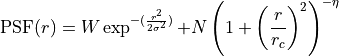
Parameters:

• r (float or array) – The radial distance from the true source position is arcsec.

• W (float) – Normalization of the Gaussian component.

• sigma (float) – Width of the Gaussian component.

• N (float) – Normalization of the King component.

• r_c (float) – Characteristic radius of the King component.

• eta (float) – Exponent of the King component.

ixpeobssim.irf.psf.gauss_king_eef_at_infinity(W, sigma, N, r_c, eta)

Return the value of the Encircled Energy Fraction (EEF) at infinity, given the parameters of the functional representation, see equation (4) of Fabiani et al., 2014.

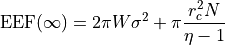
Parameters:

• r (float or array) – The radial distance from the true source position is arcsec.

• W (float) – Normalization of the Gaussian component.

• sigma (float) – Width of the Gaussian component.

• N (float) – Normalization of the King component.

• r_c (float) – Characteristic radius of the King component.

• eta (float) – Exponent of the King component.

class ixpeobssim.irf.psf.xPointSpreadFunction(file_path)

Class describing a (simplified, energy independent) PSF.

The effective area is essentially a linear spline, with built-in facilities for evaluation and plotting.

Parameters:

psf_file_path (str) – The path to the .psf FITS file containing the PSF parameters.

Note

The parametrization is taken from Fabiani et al., 2014, table 2.

build_eef()

Build the Encircled Energy Fraction (EEF) as a function of r.

And, while we’re at it, we also calculate and cache the HEW.

delta(size=1)

Return an array of random offset (in ra, dec or L, B) due to the PSF.

Note the output is converted in degrees.

draw_psf_circle(image, x=0.8, y=0.8, label='HPD', hpd_value=False, color='white', lw=1.5)

Add the PSF circle to the image with labels.

Parameters:

• image (xFITSImageBase instance) – The parent xFITSImageBase object

• x (float) – The position of the psf circle in relative canvas coordinates

• y (float) – The position of the psf circle in relative canvas coordinates

plot()

Overloaded plot method.

class ixpeobssim.irf.psf.xPointSpreadFunction2d(file_path)

Two-dimensional version (i.e., non azimuthally symmetric) version of the PSF.

Parameters:

file_path (str) – The file path for the PSF image

build_eef()

Calculate the (azimuthally averaged) encircled energy fraction as a function of r.

delta(size=1)

Return an array of random offset (in ra, dec) due to the PSF.

class ixpeobssim.irf.psf.xPointSpreadFunctionBase(gpd)

Base virtual class for the PSF data structures.

New in version 28.1.0: This was added in version 27.1.0 as a base class for the old-style PSF (azimuthally symmetric and including the position resolution of the GPD) and the new-style PSF necessary to study the Stokes cross-talk (non azimuthally symmetric and limited to the X-ray optics).

This class holds a single boolean flag inficating whether the GPD position resolution is included in the PSF. Sub-classes should reimplement the delta() hook, returning random arrays of (ra, dec) offsets.

Parameters:

gpd (bool) – Boolean flag indicating whether a given PSF includes the effect of the GPD position resolution.

delta(size=1)

Return an array of random offset (ra, dec) due to the PSF.

smear(ra, dec)

Smear a pair of arrays of coordinates.

smear_single(ra, dec, size=1)

Smear a single pair of coordinates for an arbitrary number of times.

Definition of the response matrix.

class ixpeobssim.irf.rmf.xEnergyDispersion(file_path)

Class representing the energy dispersion.

Parameters:

file_path (str) – The path to the .rmf FITS file containing the energy dispersion tables.

channel_to_energy(channel)

Convenient proxy to the underlying xEnergyDispersionBounds method.

convolve_energy(mc_energy)

Convolve an array of mc_energy with the energy dispersion.

This function is less trivial than the name might suggest, and it is performing several different operations at the same time, namely:

• call xEnergyDispersionMatrix.rvs2() to smear the true energy and get the measured energy (in channel space) both before and after the digitization;

• convert the measured energy before digitization to keV;

• convert the pha to pulse invariant.

energy_to_channel(energy)

Convenient proxy to the underlying xEnergyDispersionBounds method.

pha_analysis(energy)

Perform a pulse-height analysis on a given array of energies.

static pha_to_pi(pha)

Simple placeholder method to convert a PHA value to pulse invariant.

Note

Since we’re not handling the gain corrections, yet, this is simply converting the values from integer to floating point numbers.

plot()

Plot the energy dispersion.

static scale_energy(energy)

Hook to allow to apply distorsions to the energy response of the detector.

In this default implementation this is just returning the energy, untouched, but the method can be overridden to simulate a variety of systematic effects.

class ixpeobssim.irf.rmf.xEnergyDispersionBounds(hdu)

Class encapsulating the bounds for the energy dispersion matrix, as stored in the EBOUNDS extension of a .rmf file.

This is essentially a univariate spline with the channel number on the x axis and the average energy of the corresponding interval on the y axis. At the same time we do store the bounds of the intervals themselves.

channel_to_energy(channel)

Convert a channel number to energy.

energy_to_channel(energy)

Convert a physical energy (in keV) into a channel number.

This is using a simple binary search on the underlying energy bounds.

max()

Return the maximum energy of the last channel.

min()

Return the minimum energy of the first channel.

num_channels()

Return the number of channels.

class ixpeobssim.irf.rmf.xEnergyDispersionMatrix(hdu)

Class encapsulating the energy dispersion matrix, as stored in the MATRIX extension of a .rmf file.

We don’t downsample the matrix to avoid the failure of the fit procedure in XSPEC.

Parameters:

hdu (FITS hdu) – The MATRIX hdu in the .rmf FITS file.

static digitize(value, dtype=<class 'numpy.int16'>)

Digitize an energy value.

This is essentially rounding an array to the nearest integer and cast the result to the specified type.

rvs(aux)

Overloaded method.

This is the original rvs() overloade method that was initially implemented in the energy dispersion code, and it is digitizing the measured energy before returning it, just like the detector would do in real life.

We discovered along the way that it is handy to keep track of the measured (smneared) energy before the digitization (i.e., with all the significant digits), as this allows to apply corrections (e.g., for the GEM charging) without running into rounding problems. This is why we added the rvs2() class method, which is returning both.

rvs2(aux)

Alterntative rvs() implementation where we return the measured energy both before and after the digitization.

Note that the energy before the digitization is still in the pha space, and needs to be explicitely converted to physical units (keV), if that it what one is interested. When that’s the case, the operation is deferred to the xEnergyDispersion class, who is aware of both the energy dispersion matric and the energy bounds.

PSF parametrization.

class ixpeobssim.irf.vign.xVignetting(file_path)

Class describing vignetting.

The vignetting is essentially a bivariate linear spline, with built-in facilities for evaluation and plotting.

Parameters:

file_path (str) – The path to the vign.fits file containing the vignettting table.

plot()

Plot the vignetting.

IRF Generation

Small module providing simulation tools for the alpha particles emitted by the Be window.

ixpeobssim.irfgen.alphas.gas_cell_intersection_points(ray)

Calculate the intersecting points of a given ray with the gas cell.

This is a horrible list of conditions, and should be

ixpeobssim.irfgen.alphas.generate_decays(alpha_energy=5.0, num_alphas=1000000, plot=True, energy_cut=0.1)

Generate the initial alpha particles in the Be window volume.

This is returning a list of xRay object and a numpy array of energies describing the alpha particles that emerge from the window in a direction that is intersecting the fiducial cylinder enclosing the GPD active gas volume.

This first part of the program is vectorized, as only a small fraction of the particles survive the initial cut, and the whole thing would be excruciatingly slow, if stuffed into a plain Python loop.

ixpeobssim.irfgen.alphas.generate_distributions(alpha_energy=5.0, num_alphas=10000000)

ixpeobssim.irfgen.alphas.plot_distributions(alpha_energy=5.0, num_alphas=1000000)

ixpeobssim.irfgen.alphas.plot_event(ray, enery, track_start=None, track_end=None)

Rudimentary single-event display.

ixpeobssim.irfgen.alphas.plot_raindrops(alpha_energy=5.0, num_alphas=2000, max_roi_size=5000)

ixpeobssim.irfgen.alphas.plot_rectangle(width, height, center=(0.0, 0.0), **kwargs)

Facility to plot a generic rectangle.

ixpeobssim.irfgen.alphas.simulate(alpha_energy=5.0, num_alphas=100000, plot=False, energy_cut=0.1)

Run the actual simulation.

ixpeobssim.irfgen.astar.load_alpha_stopping_power_data(identifier, density=None)

Load the stopping power data for a given element or compound.

ixpeobssim.irfgen.astar.load_dme_alpha_stopping_power_data(temperature=20.0, pressure=800.0)

Load the stopping power data for a given element or compound.

class ixpeobssim.irfgen.astar.xAlphaStoppingPowerTable(identifier, density=None)

Basic interface to the output files of the ASTAR database.

bragg_curve(energy=10.0, energy_step=0.01)

Return a spline representing the Bragg curve for the element or compound.

energy_loss(max_energy=10.0, energy_step=0.01)

process_data()

Do all the post-processing of the underlying data.

class ixpeobssim.irfgen.astar.xDMEAlphaStoppingPowerTable(temperature, pressure)

Specialized subclass for the DME compound.

Library for producing auxiliary files for the IRF generation.

ixpeobssim.irfgen.auxiliary.absorption_type_masks(mc_absz, min_dme_absz=0.832, max_dme_absz=10.83)

Return a set of three masks for the window, DME and GEM absorption.

This is based on the Monte Carlo z coordinate of the absorption point, and it is not the most elegant solution, as the correctness of the mask relies on the fact that we use the right bounds for the thickness of the absorption gap used in the simulations. (Since the latter is essentially never changed, this is less horrible than it might seems at a first glance.)

Moving forward, fixing https://bitbucket.org/ixpesw/gpdsw/issues/222 and use the exact information might be the way to go.

ixpeobssim.irfgen.auxiliary.allx_edisp_file_path(abs_label, weight_name, aux_version=3)

Return the path to the allx edisp data file path for a given absorption type and set of weights.

ixpeobssim.irfgen.auxiliary.allx_pha_model_file_path(aux_version=3)

Return the path to the file with the PHA model.

ixpeobssim.irfgen.auxiliary.allx_qeff_file_path(weight_name, aux_version=3)

Return the path to the allx lines data file path for a given absorption type and set of weights.

ixpeobssim.irfgen.auxiliary.allx_rmf_file_path(abs_label, weight_name=None, aux_version=3)

Return the path to the FITS file(s) to be used to compose the response matrix.

ixpeobssim.irfgen.auxiliary.calculate_efficiency(n, N)

Calculate the efficiency, given a number of trials and success, and attach the classical binomial error to it.

ixpeobssim.irfgen.auxiliary.calculate_pi(mc_energy, pha)

Perform the conversion from PHA to PI.

This is necessary because the PHA values in the ixpesim simulation are expressed in the terms of the native detector ADC counts, and the scale factor to the actual energy channels in the response functions is arbitrary. In real life the conversion will be based on the ground calibration with monochromatic sources, and this is meant to be a sensible proxy for that process for operating on Monte Carlo data sets.

Note this operates differently depending on whether we’re working with line data or a continoum spectrum.

Parameters:

• mc_energy (array_like) – The array of (true) energies in keV

• pha (array_like) – The array of measured PHA values.

Returns:

• rec_energy (array_like) – The array of reconstructed energies (in keV) corresponding to the input PHAs.

• pi (array_like) – The array of pulse invariants corresponding to the input PHAs.

• pha_model (xInterpolatedUnivariateSpline object) – The model to operate the conversion between PHAs and PIs.

ixpeobssim.irfgen.auxiliary.calculate_pi_broadband(mc_energy, pha, energy_binning=None)

Calculate the event pulse invariant for a broadband simulation.

This is trying to account for the bulk of the non linearities by fitting the normalized PHA in different energy slices and then fitting the scale factor as a function of the energy with an erf function. (The effect is of the order of 2% from 2 keV to 12 keV, at about 3000 ADC counts per keV nominal.)

ixpeobssim.irfgen.auxiliary.calculate_pi_line(pha, aux_version=3)

Convert the pha column into pulse invariant for a line simulation.

Note that, for line simulations, we use the PHA model derived from the allx data set.

ixpeobssim.irfgen.auxiliary.event_weights(event_data, label='alpha075')

Book-keeping function mapping text labels to weights.

ixpeobssim.irfgen.auxiliary.lines_edisp_file_path(abs_label, weight_name, aux_version=3)

Return the path to the lines edisp data file path for a given absorption type and set of weights.

ixpeobssim.irfgen.auxiliary.lines_qeff_file_path(weight_name, aux_version=3)

Return the path to the lines qeff data file path for a given absorption type and set of weights.

ixpeobssim.irfgen.auxiliary.lines_rmf_file_path(abs_label, weight_name=None, aux_version=3)

Return the path to the FITS file(s) to be used to compose the response matrix.

ixpeobssim.irfgen.auxiliary.load_allx_edisp_data(abs_label, weight_name=None, aux_version=3)

Load the (raw) response matrix data created with mkauxallx.py.

ixpeobssim.irfgen.auxiliary.load_allx_rmf_hist(abs_label, weight_name=None, aux_version=3)

Load the post-processed histogram with the rmf data.

ixpeobssim.irfgen.auxiliary.load_event_data(*file_list, absorption_masks=True, pi=True)

Load the data from the (reconstructed) event files generates with ixpesim.

This is chaining together all the data in the input files—for allx simulations you should pass all the files to a single function call, while for lines you should be open them one by one.

The event data are returned in the form of a dictionary indexed by the corresponding column names in the EVENTS and MONTE_CARLO extensions of the photon lists. Metadata are stored into a separate info dictionary.

ixpeobssim.irfgen.auxiliary.load_lines_edisp_data(abs_label, weight_name=None, aux_version=3)

Load the quantum efficiency data from file.

ixpeobssim.irfgen.auxiliary.load_lines_rmf_hist(abs_label, weight_name=None, aux_version=3)

Load the post-processed histogram with the rmf data.

ixpeobssim.irfgen.auxiliary.load_pha_model(aux_version=3)

Load a PHA to PI model from file.

ixpeobssim.irfgen.auxiliary.load_pressure_scan_table(file_path, col_name='MU2')

Load the pressure scan data from file.

This is reading the binary table stored in the FITS files and arranging them in an order that is suitable for interpolation in pressure and energy.

ixpeobssim.irfgen.auxiliary.load_qeff_table(file_path)

Load the quantum efficiency data from file.

This is reading the binary table stored in the FITS files and returning the columns in the form of a Python dictionary indexed by column name.

ixpeobssim.irfgen.auxiliary.pscan_modf_file_path(weight_name, aux_version=3)

Return the path to the modulation factor data from the analysis of the pressure scan.

ixpeobssim.irfgen.auxiliary.write_pha_model(file_path, model, info)

Write the PHA to PI conversion model table to file.

ixpeobssim.irfgen.auxiliary.write_pressure_scan_table(file_path, data, info)

Write a pressure table to file.

ixpeobssim.irfgen.auxiliary.write_qeff_table(file_path, data, info)

Write a quantum efficiency table to file.

class ixpeobssim.irfgen.auxiliary.xEdispModelGenGauss

Energy dispersion fitting model.

This is the combination of a generalized Gaussian distribution for the main peak, and a hat-shaped bridge for the tail, with the possible addition of a low-energy bump.

static value(x, norm, peak_frac, peak, sigma, beta, bump_frac)

Overloaded value() method.

class ixpeobssim.irfgen.auxiliary.xEdispModelLogNormal

Energy dispersion fitting model.

This is the combination of a log-normal distribution for the main peak, and a hat-shaped bridge for the tail, with the possible addition of a low-energy bump.

static value(x, norm, peak_frac, peak, sigma, shape, endpoint, bump_frac, bump_sigma)

Overloaded value() method.

Base module for all the facilities related to the creation of response functions.

ixpeobssim.irfgen.base.make_arf(irf_name, du_id, pressure, creator, comments, weight_name=None, aux_version=3)

Write the IXPE effective area response function.

ixpeobssim.irfgen.base.make_modf(irf_name, du_id, pressure, creator, comments, weight_name=None, aux_version=3)

Write the IXPE modulation factor response function.

ixpeobssim.irfgen.base.make_mrf(irf_name, du_id, pressure, creator, comments, weight_name=None, aux_version=3)

Write the IXPE effective area response function.

ixpeobssim.irfgen.base.make_psf(irf_name, du_id, params, creator, comments, weight_name=None, aux_version=3)

Write the IXPE PSF response function.

ixpeobssim.irfgen.base.make_rmf(irf_name, du_id, pressure, creator, comments, weight_name=None, aux_version=3)

Write the IXPE edisp response function.

The specifications are described at page ~15 of the following document: ftp://legacy.gsfc.nasa.gov/caldb/docs/memos/cal_gen_92_002/cal_gen_92_002.ps

ixpeobssim.irfgen.base.make_vign(irf_name, du_id, pressure, creator, comments, weight_name=None, aux_version=3)

Write the IXPE vignetting response function.

ixpeobssim.irfgen.du.uv_filter_transparency(energy)

Return the transparency of the UV filter evaluated on a given grid of energy points.

ixpeobssim.irfgen.du.uv_filter_transparency_spline()

Return a spline with the transparency of the UV filter as a function of the energy.

ixpeobssim.irfgen.gpd.dme_photoemission_frac_spline(pressure=800.0)

Return a spline representing the fraction of photoelectons extracted from the DME as a function of energy.

This is achieved by calculating the probability of extracting a photoelectron from the Be window and the GEM using the Geant 4 Monte Carlo simulation.

ixpeobssim.irfgen.gpd.load_ixpesim_ancillary_data(file_name='ixpesim_stdlines_20191109.txt')

Load the ancillary data calculated with the full Geant 4 Monte Carlo simulation to inform the generation of the instrument response functions.

The columns represent, in order:

• Energy [keV];

• Trigger efficiency;

• Probability of extraction of a photoelectron from the Be window;

• Probability of extraction of a photoelectron from the GEM Cu upper layer;

• Simulated value of the modulation factor.

ixpeobssim.irfgen.gpd.modulation_factor(energy, pressure, weight_name=None, aux_version=3)

Return the modulation factor calculated on a grid of points.

ixpeobssim.irfgen.gpd.photoabsorption_efficiency(energy, temperature, pressure, thickness=1.0)

Return the photoabsorption efficiency of the GPD absorption gap.

ixpeobssim.irfgen.gpd.quantum_efficiency(energy, temperature, pressure, weight_name=None, aux_version=3)

Return the overall quantum efficiency of the GPD.

Parameters:

• energy (array-like) – The energy array where the quantum efficiency is calculated

• temperature (float) – The GPD filling temperature

• pressure (float) – The GPD gas pressure

• weight_name (str) – The label for the weights to be used.

• aux_version (int) – The version of the auxiliary data products used to model the passive conversions.

ixpeobssim.irfgen.gpd.window_al_transparency(energy, thickness=5.3e-06)

Return the transparency of the 53 nm alumination of the Be window.

ixpeobssim.irfgen.gpd.window_be_transparency(energy, contaminants={'Ag': 10.0, 'Al': 300.0, 'B': 3.0, 'BeO': 6000.0, 'C': 400.0, 'Ca': 100.0, 'Cd': 2.0, 'Co': 10.0, 'Cr': 100.0, 'Cu': 100.0, 'Fe': 800.0, 'Li': 3.0, 'Mg': 490.0, 'Mn': 100.0, 'Mo': 20.0, 'Ni': 100.0, 'Pb': 20.0, 'Si': 300.0, 'Th': 2.0, 'U': 140.0}, thickness=0.005)

Return the transparency of the 50 um Be window.

Parameters:

• energy (array-like) – The array of energy values where we calculate the transparency.

• contaminants (dict, optional) – A dictionary containing the list and concentration of contaminants in the Be window.

ixpeobssim.irfgen.gpd.window_transparency(energy, contaminants={'Ag': 10.0, 'Al': 300.0, 'B': 3.0, 'BeO': 6000.0, 'C': 400.0, 'Ca': 100.0, 'Cd': 2.0, 'Co': 10.0, 'Cr': 100.0, 'Cu': 100.0, 'Fe': 800.0, 'Li': 3.0, 'Mg': 490.0, 'Mn': 100.0, 'Mo': 20.0, 'Ni': 100.0, 'Pb': 20.0, 'Si': 300.0, 'Th': 2.0, 'U': 140.0})

Return the overall window transparency.

class ixpeobssim.irfgen.gpd.xEdispDataInterface(weight_name=None, aux_version=3)

Basic interface to the post-processed ixpesim output that is necessary to create the response matrix.

combine(temperature=20.0, pressure=800.0, contaminants={'Ag': 10.0, 'Al': 300.0, 'B': 3.0, 'BeO': 6000.0, 'C': 400.0, 'Ca': 100.0, 'Cd': 2.0, 'Co': 10.0, 'Cr': 100.0, 'Cu': 100.0, 'Fe': 800.0, 'Li': 3.0, 'Mg': 490.0, 'Mn': 100.0, 'Mo': 20.0, 'Ni': 100.0, 'Pb': 20.0, 'Si': 300.0, 'Th': 2.0, 'U': 140.0})

Combine the window, DME and GEM response functions in the proper proportions (depending on the target temperature and pressure, as well as the window contaminants) to create the actual response function.

class ixpeobssim.irfgen.gpd.xModfDataInterface(weight_name=None, aux_version=3)

Basic interface to the post-processed ixpesim output parametrizing the modulatuion factor as a function of the pressure.

pressure_slice(pressure)

Return a slice at the given pressure, in the form of a piecewise interpolated spline.

class ixpeobssim.irfgen.gpd.xQeffDataInterface(weight_name=None, aux_version=3)

Basic interface to the post-processed ixpesim output that is necessary to create the arf response functions.

This is essentially reading the FITS file with the quantum efficiency tabulated as a function of the energy for the different conversion types (window, DME, and GEM) and caching the necessary arrays in a form that is convenient for later use.

In addition, the class is parametrizing the extraction probabilities for the window and the GEM, so that we can readily scale all the relevant quantities at different internal pressure in a self-consistent fashion without the need to re-run the original simulations.

Warning

When we updated this to allow for weights, it became clear that the efficiency of the active gas volume could not be simply computed from the analystic formula (which was the original approach).

We therefore decided to cache the (energy-dependent) weighting efficiency along with the other quantities, based on the consideration that its dinamic range is comparatively small, and it is therefore more easily amenable to interpolation.

dme_absorption_prob(energy, temperature=20.0, pressure=800.0, contaminants={'Ag': 10.0, 'Al': 300.0, 'B': 3.0, 'BeO': 6000.0, 'C': 400.0, 'Ca': 100.0, 'Cd': 2.0, 'Co': 10.0, 'Cr': 100.0, 'Cu': 100.0, 'Fe': 800.0, 'Li': 3.0, 'Mg': 490.0, 'Mn': 100.0, 'Mo': 20.0, 'Ni': 100.0, 'Pb': 20.0, 'Si': 300.0, 'Th': 2.0, 'U': 140.0})

Return the probabilty for a photon of being absorbed in the DME at a given energy (or array of energies).

dme_quantum_efficiency(energy, temperature=20.0, pressure=800.0, contaminants={'Ag': 10.0, 'Al': 300.0, 'B': 3.0, 'BeO': 6000.0, 'C': 400.0, 'Ca': 100.0, 'Cd': 2.0, 'Co': 10.0, 'Cr': 100.0, 'Cu': 100.0, 'Fe': 800.0, 'Li': 3.0, 'Mg': 490.0, 'Mn': 100.0, 'Mo': 20.0, 'Ni': 100.0, 'Pb': 20.0, 'Si': 300.0, 'Th': 2.0, 'U': 140.0})

Return the quantum efficiency of the DME.

gem_absorption_prob(energy, temperature=20.0, pressure=800.0, contaminants={'Ag': 10.0, 'Al': 300.0, 'B': 3.0, 'BeO': 6000.0, 'C': 400.0, 'Ca': 100.0, 'Cd': 2.0, 'Co': 10.0, 'Cr': 100.0, 'Cu': 100.0, 'Fe': 800.0, 'Li': 3.0, 'Mg': 490.0, 'Mn': 100.0, 'Mo': 20.0, 'Ni': 100.0, 'Pb': 20.0, 'Si': 300.0, 'Th': 2.0, 'U': 140.0})

Return the probabilty for a photon of being absorbed in the GEM at a given energy (or array of energies).

gem_extraction_prob(energy)

Return the photoelectron extraction probability for the GEM at a given energy.

Mind we clip the output of the spline interpolation to the [0, inf] interval, as the spline might accidentally go below zero at low energy due to the noise.

gem_quantum_efficiency(energy, temperature=20.0, pressure=800.0, contaminants={'Ag': 10.0, 'Al': 300.0, 'B': 3.0, 'BeO': 6000.0, 'C': 400.0, 'Ca': 100.0, 'Cd': 2.0, 'Co': 10.0, 'Cr': 100.0, 'Cu': 100.0, 'Fe': 800.0, 'Li': 3.0, 'Mg': 490.0, 'Mn': 100.0, 'Mo': 20.0, 'Ni': 100.0, 'Pb': 20.0, 'Si': 300.0, 'Th': 2.0, 'U': 140.0})

Return the quantum efficiency of the GEM.

Note that, while the GEM extraction probability is pressure-independent, this depends on the pressure due to the effect of the absorptions in the gas, changing the number of X-ray photons reaching the GEM top.

plot_extraction_probability()

Plot the probability of extracting a photoelectron from either the window or the GEM as a function of energy.

plot_quantum_efficiency(temperature=20.0, pressure=800.0)

Plot the quantum efficiency as a function of the energy, disaggregated by conversion type.

quantum_efficiency(energy, temperature=20.0, pressure=800.0, contaminants={'Ag': 10.0, 'Al': 300.0, 'B': 3.0, 'BeO': 6000.0, 'C': 400.0, 'Ca': 100.0, 'Cd': 2.0, 'Co': 10.0, 'Cr': 100.0, 'Cu': 100.0, 'Fe': 800.0, 'Li': 3.0, 'Mg': 490.0, 'Mn': 100.0, 'Mo': 20.0, 'Ni': 100.0, 'Pb': 20.0, 'Si': 300.0, 'Th': 2.0, 'U': 140.0})

Return the ovearall GPD quantum efficiency, including all the absoprtion types.

weight_eff_dme(energy)

Return the DME weighting efficiency at a given array of energies.

weight_eff_gem(energy)

Return the GEM weighting efficiency at a given array of energies.

weight_eff_win(energy)

Return the window weighting efficiency at a given array of energies.

window_absorption_prob(energy, temperature=20.0, pressure=800.0, contaminants={'Ag': 10.0, 'Al': 300.0, 'B': 3.0, 'BeO': 6000.0, 'C': 400.0, 'Ca': 100.0, 'Cd': 2.0, 'Co': 10.0, 'Cr': 100.0, 'Cu': 100.0, 'Fe': 800.0, 'Li': 3.0, 'Mg': 490.0, 'Mn': 100.0, 'Mo': 20.0, 'Ni': 100.0, 'Pb': 20.0, 'Si': 300.0, 'Th': 2.0, 'U': 140.0})

Return the probabilty for a photon of being absorbed in the window at a given energy (or array of energies).

window_extraction_prob(energy)

Return the photoelectron extraction efficiency for the Be window at a given energy.

Mind we clip the output of the spline interpolation to the [0., 1.] interval, as the spline might accidentally go below zero at low energy due to the noise.

window_quantum_efficiency(energy)

Another name for the same thing :-)

The window sees all the photons we generate with ixpesim, so the denominator is 1, and the quantum efficiency is exactly equal to the extraction probability.

ixpeobssim.irfgen.xcom.create_energy_grid(emin=0.001, emax=0.015, num_points=100)

Create a text file with a list of additional energies to query the XCOM databse, to be passed to the XCOM web interface.

By default this is writing out a grid of logarithmically-spaced energy values between 1 and 15 keV—one energy per line, in MeV.

ixpeobssim.irfgen.xcom.load_xsection_data(identifier)

Load the cross-section data for a given element or compound.

Source Models

Background model components.

class ixpeobssim.srcmodel.bkg.xCelestialBkgBase(name, ra, dec, photon_spectrum, identifier=None)

Base class for the celestial background components.

Celestial background is assumed to be uniform within the field of view, and is therefore modeled as a uniform disk with a radius larger than the field of view itself—the normalization should be computed self-consistently for the full disk, and when the GPD fiducial cut is applied the photons that do not hit the detector are simply thrown away.

(Other than the fact that the normalization is normalized to the solid angle of the component, this is essentially identical to any other celestial component.)

Note that, by construction, the component is unpolarized, and the column density and redshift are identically zero.

static solid_angle(radius)

Return the solid angle subtended by a cone of aperture radius.

See https://en.wikipedia.org/wiki/Solid_angle

Parameters:

radius (float) – The half-apex of the cone in decimal degrees.

class ixpeobssim.srcmodel.bkg.xExtragalacticBkg(ra, dec, identifier=None)

Derived class for the extragalactic X-ray background.

All the basic formalism is taken from Gruber et al., 1999 https://iopscience.iop.org/article/10.1086/307450/pdf

Essentially in our energy band we model the extragalactic background as a broken power law with index 1.29 and break energy 41.13 keV.

Note 1.29 is the index of the photon spectrum, while the 0.29 in the paper refers to the energy spectrum, see https://bitbucket.org/ixpesw/ixpeobssim/issues/544

class ixpeobssim.srcmodel.bkg.xGalacticBkg(ra, dec, rosat_r7_bkg_rate, identifier=None)

Derived class for the galactic X-ray background.

A good reference for this is Tanaka, 2002: https://www.aanda.org/articles/aa/pdf/2002/06/aah3204.pdf

Operationally, I think the most convenient mean to gauge the intensity of the Galactic background is the HEASARC background tool https://heasarc.gsfc.nasa.gov/cgi-bin/Tools/xraybg/xraybg.pl and, particularly, the ROSAT count rate in the 1–2 keV energy band (R7).

class ixpeobssim.srcmodel.bkg.xInstrumentalBkg(name, photon_spectrum, radial_slope=0.0, identifier=None, convolve_energy=False)

Base class for the instrumental background

In addition to the base class xModelComponentBase, this class has the spectrum member to fully describe the spectrum of the instrumental background.

This essentially corresponds to a uniform, unpolarized source in the GPD reference frame, whose events are not convolved with any of the instrument response functions, except for the energy dispersion, if explicitely requested.

Parameters:

• name (str) – The name of the component

• photon_spectrum (callable) – The photon spectrum in photons cm-2/s-1/keV-1 for the bkg source.

• radial_slope (float) – The radial slope for the distribution in detector coordinates.

• identifier (int, optional) – The source identifier.

• convolve_energy (bool) – Convolve the source spectrum with the energy dispersion (default is False).

rvs_event_list(parent_roi, irf_set, **kwargs)

Overloaded method.

rvs_photon_list(parent_roi, irf_set, **kwargs)

Extract a random photon list.

class ixpeobssim.srcmodel.bkg.xPowerLawInstrumentalBkg(norm=0.0004, index=1.0, radial_slope=0.0)

Specialized instrumental background source with a power-law spectrum.

The default values for the spectral parameters are set after Bunner et al. 1978 (1978ApJ…220..261B), where the authors provide the non X-ray background rates for their three detectors. We are using values for the Neon filled detector in Table 3 of the paper. We fit the three points (energy bins: 0.76–1.6, 1.6–3.0, 3.0–6.0) with a power law. The best-fit values for the index and normalization of this power-law are 1.0 and 4.e-4, respectively.

class ixpeobssim.srcmodel.bkg.xRadialBackgroundGenerator(radial_slope, num_points=100)

Univariate generator sampling the radial coordinate on the detector surface for a background component whose radial distribution, normalized by the area, depends linearly on the radius.

This was introduced in https://github.com/lucabaldini/ixpeobssim/issues/663

The need for an instrumental background component that is not uniform in detector coordinates stems from the analysis of a number of observations. Interestingly enough, the radial slope of the background counts per unit area seems to be different for different observation.

Warning

While initially I was hoping to code this by sampling two independent random variables, within the proper bounds, on the x and y coordinates, it turned out that an azimuthally symmetric bivariate pdf cannot be expressed as the product of two independent variables on a square, and we had to resort to sampling r over a circle and trimming in the fiducial rectangle after the fact. This is hugly, as we need to guess in advance how much random numbers we have to throw so that we end up with enough counts after the trimming, but so life goes.

This is essentially an univariate generator whose pdf is a slight generalization of the function f(r) = 2r (for r = 1) that one would use to throw random numbers uniformly distributed in a circle:

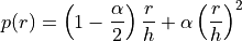
The radial slope alpha repesents the fractional half-excursion of the variation across the size h of the fiducial rectangle. For alpha = 0 the detector position are distributed uniformly over the fiducial rectangle. For alpha = 2 the radial dependence is maximal, and the density of events is zero at the center of the detector. For alpha = -1 (and assuming a square fiducial region) the pdf approaches zero at the boundary of the circle.

Parameters:

radial_slope (float) – The slope of the radial profile, that is, the fractional half-excursion of the variation across the size of the fiducial rectangle.

static average_oversample_fraction(radial_slope)

Return an heuristic for the average oversample fraction for a given radial slope of the profile.

This is a purely geometric factor that is easy to calculate for a flat profile (slope = 0), in which case it reads pi/2 but not trivial in the general case. Our approach is to generate events within the smallest circle ciscumscribed to the fiducial rectangle on a grid of radial slope values and measure the fraction that ends up in the fiducial rectangle itself. For completeness, this is calculated in tests/test_radial_bkg.py.

Note that this is accurate within a few % in the limit of infinite statistics.

oversampled_size(size, radial_slope, safety_factor=1.2, min_size=1000)

Return the oversampled size for a given target size and radial slope.

This is essentially the function that determines how many random numbers we need to throw to be sure that, after trimming to the fiducial region, we end up to enough events. This is purely heuristic and is based on the average_oversample_fraction() function when the statistics is large enough, with a minimum bound to be sure we are not killed by statistical fluctuation in the small number regime.

static pdf(r, radial_slope)

Small function encapsulating the underlying pdf for the random generator.

Note we are using the average physical size of the GPD along the x and y directions as an effective value for the radial parametrization.

static polar_to_cartesian(r, phi)

Convert an array of polar coordinates in the plane into the corresponding cartesian coordinates.

rvs_xy(size)

Extract a set of arrays of coordinate detectors.

class ixpeobssim.srcmodel.bkg.xRosatPSPCResponseMatrix

Simple interface to the ROSAT PSPC response matrix.

The FITS files was downloaded from the ROSAT HEASARC page, and the content seems qualitatively in agreement with the expectations based on the XRT collecting area https://heasarc.gsfc.nasa.gov/docs/rosat/ruh/handbook/node39.html#figXMAareas and the PSPC quantum efficiency https://heasarc.gsfc.nasa.gov/docs/rosat/ruh/handbook/node56.html#SECTION00730000000000000000

The on-axis effective area is included in the response matrix, and to extract it we just sum the (un-normalized) pdf in each energy bin.

The effective area is stored internally as an interpolated spline of order k=1.

class ixpeobssim.srcmodel.bkg.xTemplateInstrumentalBkg(file_path='/home/docs/checkouts/readthedocs.org/user_builds/ixpeobssim/checkouts/latest/ixpeobssim/srcmodel/ascii/bkg_smcx1_01903701.txt', emin=0.1, emax=15.0, k=1, radial_slope=0.0)

Instrumental background based on a template.

In-flight calibration sources and calibration-related facilities.

class ixpeobssim.srcmodel.calibsrc.xCalC(rate)

Class describing the “Cal C” onboard calibration source.

rvs_detxy(size)

Overloaded method.

class ixpeobssim.srcmodel.calibsrc.xCalibrationROIModel(source)

Class describing a custom ROI (region of interest) model for calibration sources.

In contrast to celestial ROI models, calibration ROI models only handle one source.

rvs_event_list(irf_set, **kwargs)

Extract an event list for the full ROI.

class ixpeobssim.srcmodel.calibsrc.xCalibrationSourceBase(rate)

Base class for all (on-ground and on-orbit) calibration sources.

The common denominator to all the calibration sources is:

• the event rate is constant in time and the counting statistics is Poisson;

• a specific identifier (>=100) is assigned to each source, and set once and for all, independently on the ROI machinery (this is different from the celestial sources, where the identifier is typically assigned depending on the order in which the ROI is populated);

• there is no concept of parent ROI, as the calibration sources are supposed to be operated one at a time, and independently from the satellite pointing;

• there is no concept of GTI, the start_met and duration being literally all we care about when it comes to decide whether the source is activated or not.

rvs_detphi(size)

Extract the photoelectron emission direction in detector coordinates.

Do-nothing method to be re-implemented in derived classes.

rvs_detxy(size)

Extract the event positions in detector coordinates.

Do-nothing method to be re-implemented in derived classes.

rvs_energy(size)

Extract the event energies.

Do-nothing method to be re-implemented in derived classes.

rvs_event_list(irf_set, **kwargs)

Main interface to generate random events from the calibration source.

Note that the signature here is different from the celestial sources, as we don’y need the reference to the parent ROI.

Also, since the calibration sources are not meant to be combined, the deadtime and the trigged id are calculated right away in the body function.

rvs_time(start_met, duration)

Extract the event times.

Here we essentially throw a random number with a Poisson distribution based on the expected mean of events, and then extract the event times at random—uniformly distributed between the start and stop met.

This is supposed to be the common paradigm for all the calibration sources.

class ixpeobssim.srcmodel.calibsrc.xCalibrationSourceImage(file_path)

Small convenience class descring the morphology of a calibration source in detector coordinates.

Warning

This functionality has significant overlap with the xFITSImage class in srcmodel.roi and the two should be refactored. Also: the very concept of a map in detector coordinates stored in the form of a FITS file has a lot in common with the stuff on the spurious modulation branch, and all of these things should be accommodated in a consistent fashion.

The HALF_SIDE top-level class member was added in response to issue https://github.com/lucabaldini/ixpeobssim/issues/668 and was set to the old value of the fiducial half-side. This is now self-contained to the calibration source machinery, and we might have to generalize the code to arbitrary fiducial cuts in the future, if we ever want to heavily use this functionality (which has not been the case, up to now).

plot()

Plot the source image.

rvs_coordinates(size=1)

Generate random coordinates based on the image map.

class ixpeobssim.srcmodel.calibsrc.xMonochromaticUnpolarizedCalibrationSourceBase(rate, energy)

Specialized base class for monochromatic unpolarized calibration sources.

rvs_detphi(size)

Overloade method.

rvs_detxy(size)

Do-nothing method to be re-implemented in derived classes.

rvs_energy(size)

Overloade method.

class ixpeobssim.srcmodel.calibsrc.xMonochromaticUnpolarizedFlatField(rate, energy)

Unpolarized square flat field at a given energy.

rvs_detxy(size)

Overloaded method.

Module containing ephemeris utilities, classes and functions

ixpeobssim.srcmodel.ephemeris.get_earth_barycentric_ephemeris(met)

Return earth barycentric vector given a set of terrestrial times referred to MET in seconds.

Parameters:

met (array_like) – Array of terrestrial times in MET

Returns:

Return the earth barycentric vector

Return type:

array

ixpeobssim.srcmodel.ephemeris.get_eccentric_anomaly(t_, orb_eph, periods=100, samples=10, plot=False)

At different time of emission of pulsar we calculate eccentric anomaly of binary system.

Eccentric Anomaly in radiants.

Parameters:

• t (array float) – Array of times at which evaluate the eccentric anomaly

• orb_eph (class xOrbitalEphemeris) – Orbital ephemeris

• periods (int) – Number of periods to use to evaluate the eccentric anomaly

• samples (int) – Number of bins in the eccentric anomaly evaluation

• plot (Boolean) – If True plot the inverse function

Returns:

returns the eccentric anomaly as a function of pulsar emission time

Return type:

class spline

ixpeobssim.srcmodel.ephemeris.phase_function(met, met0, nu0, nudot0=0.0, nuddot=0.0)

Return the rotational phase for a given observational time.

Warning

This function is deprecated in favor of the xEphemeris.met_to_phase() class method, and is (temporarily) kept for backward compatibility.

ixpeobssim.srcmodel.ephemeris.read_par_file(parfile_path)

Method to read a parameter file and to get pulsar parameters.

The following parameters are accepted:

• PEPOCH Epoch of period/frequency (MJD)

• POSEPOCH Epoch of position measuremet (MJD)

• F0 Pulsar rotation frequency (s^-1)

• F1 Pulsar rotation frequency derivative (s^-2)

• F2 Pulsar rotation frequency second derivative (s^-3)

• P0 Pulsar period (s).

• P1 Pulsar period derivative (10^-15).

• DM Dispersion measure (pc cm^-3)

• A1 Projected pulsar semi-major axis of orbit (lt-s)

• E/ECC Eccentricity of orbit

• T0 Epoch of periastron passage of orbit (MJD)

• TASC Epoch of ascending node passage (MJD)

• PB Period of orbit (days)

• OM Longitude of periastron passage (deg)

• EPS1 First Laplace parameter [E x sin(OM)]

• EPS2 Second Laplace parameter [E x cos(OM)]

• EPS1DOT Time derivative of EPS1

• EPS2DOT Time derivative of EPS2

• OMDOT Rate of periastron advance (deg/yr)

• PBDOT Rate of change of orbital period

• XDOT Rate of change of projected semi-major axis

• ECCDOT Rate of change of eccentricity

For further information refer to the TEMPO2 user manual.

Note

Parameter files are commonly used in pulsar timing analysis, because they contain precise information about pulsar position, spin-down rate, orbital parameters (if in binary systems), etc. The structure matches with a dictionary fill-in method.

Parameters:

parfile_path (str) – Path to the .par file containing the ephemeris

Returns:

Return a dictionary containing the pulsar parameters

Return type:

dictionary

ixpeobssim.srcmodel.ephemeris.time_list(pulse_shape, start_met, ephemeris, n_events, duration)

Time events extracted with the acceptance rejection method.

Parameters:

• pulse_shape – Pulse profile shape from pulse_pol_from_harmonics_spline in ixpeobssim.srcmodel.polarization

• start_met (float) – Starting time

• ephemeris (xOrbitalEphemeris object) – The orbital ehemeris to be used.

• n_events (integer) – Number of events to simulate

• duration (float) – Time of observation

class ixpeobssim.srcmodel.ephemeris.xEphemeris(met0, nu0, nudot0=0.0, nuddot=0.0)

Convenience class encapsulating the ephemeris for a periodic source.

This is meant to capture effects up to the second time derivative of the frequency.

The basic task of the class is to handle the conversion from mission elapsed time to phase and vice versa. This is performed through the met_to_phase(), and phase_to_met() interfaces. Note that, in this context, by phase we mean a free-running quantity, while by pulse phase we mean the fractional part of the former, in the [0, 1[ interval.

The direct transformation (met to phase or pulse phase) is performed through a simple taylor expansion

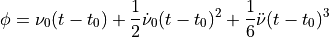
while the inverse (phase to met) is done through an interpolating spline.

In addition, given a pulse shape in the form of a xUnivariateGenerator, the class is able to extract a set of random arrays of met and pulse phase via the rvs() method. This is used in ixpeobssim.srcmodel.roi for simulating periodic sources.

Parameters:

• met0 (float) – The reference mission elapsed time.

• nu0 (float) – Rotational frequency at met0.

• nudot0 (float) – First detivative of the rotational frequency at met0.

• nuddot (float) – Second derivative of the rotational frequency (constant).

dict()

Return the ephemeris content in the form of a dictionary.

This is useful, e.g., when calling xpphase passing an ephemeris object to set the fields programmatically. The reason why we’re wrapping this and not using __dict__ directly is to be able to accommodate possible future changes in either the class layout or the options for the external programs.

fold(met, start_met, phi0=0.0)

Fold the MET values to return the corresponding arrays of pulse phase.

Warning

This is creating a new xEphemeris object with the reference MET set to start_met, and the frequency derivatives changed accordingly, and then calling the met_to_phase() method of this new object. This is supposed to roundtrip with the rvs() method to a decent accuracy, and is therefore the interface used in the xpphase application. Note, however, that there is a lot of numerical (more or less random) rounding going on under the hood, and this is not intended for “professional” use. (In a sense, the function internals are tweaked specifically for the numerical noise to play in such a way that we’re making approximately the same errors in rvs() and fold()).

classmethod from_file(parfile_path)

Read a set of attributes given a parameter file.

met_to_phase(met)

Return the phase for a given value of array of MET values.

Note the phase, here, is free-running, i.e. not bound between 0 and 1. For a simple ephemeris with zero time derivatives this is returning a straight line with a slope equal to the (constant) frequency.

nu(met)

Return the source frequency at a given time.

nudot(met)

Return the source first derivative of frequency at a given time.

period(met)

Return the source period at a given time.

phase_spline(start_met, duration, num_points=1000)

Return an interpolated univariate spline with the phase values for a given time range.

This is mainly used in the inverted fashion to convert from phase to met.

phase_spline_inverse(start_met, duration, num_points=1000)

Return the inverse of the phase spline for a given time range.

This can effectively be used for calculating the proper mission elapsed times starting from a bunch of phase values.

phase_to_met(phase, start_met=None, duration=None, num_points=1000)

Return the mission elapsed times for given value or array of phases.

This is essentially the inverse of phase(), and the two are supposed to roundtrip with each other. The reason why this function is slightly more complicated is that the former cannot be inverted analytically, and since the source frequency changes with time, it is not trivial to map directly the minimum and maximum phase to the corresponding met values, which is needed to create the interpolating spline for the conversion.

The start_met and stop_met arguments are provided to control the spline operating the conversion, and should be provided if available—in this case the span of the spline is optimal and it is guaranteed that no extrapolation is needed. Both arguments default to None, in which case a zero-order guess is made as to what their value shoule be.

Parameters:

• phase (array_like) – The phase value(s) to be converted in met.

• start_met (float) – The starting met value for the spline operating the conversion.

• duration (float) – The overall span for the spline operating the conversion.

• num_points (int) – The number of points for spline operating the conversion.

rvs(pulse_profile, start_met, duration, num_events)

Return two (sorted) arrays of pulse phase and met for a given pulse profile, observation interval and number of events.

Parameters:

• pulse_profile (xUnivariateGenerator instance) – The pulse target profile.

• start_met (float) – The initial met for the observation.

• duration (float) – The duration of the observation.

• num_events (float) – The total number of events to be simulated.

class ixpeobssim.srcmodel.ephemeris.xOrbitalEphemeris(met0, nu0, t_orbital, p_orbital, axis_proj, ecc=0.0, lon_periast=0.0, nudot0=0.0, nuddot=0.0, p_orbitaldot=0.0, eps1=None, eps2=None, model=None)

Convenience class encapsulating an orbital ephemeris.

Parameters:

• met0 (float) – Epoch of period/frequency (MET)

• nu0 (float) – Pulsar rotation frequency (s^-1)

• t_orbital (float) – Epoch of ascending node passage or Epoch of periastron passage of orbit (MET)

• p_orbital (float) – Period of orbit (s)

• axis_proj (float) – Projected pulsar semi-major axis of orbit (lt-s)

• ecc (float) – Eccentricity of orbit

• lon_periast (float) – Longitude of periastron passage (deg)

• nudot0 (float) – Pulsar rotation frequency derivative (s^-2)

• nuddot (float) – Pulsar rotation frequency second derivative (s^-3)

• p_orbitaldot (float) – Rate of change of orbital period

• eps1 (float) – First Laplace parameter [E x sin(lon_periest)]

• eps2 (float) – Second Laplace parameter [E x cos(lon_periest)]

• model (Binary model (BT/ELL1/DD/MSS)) –

classmethod from_file(parfile_path)

Read a set of attributes given a parameter file.

omega_orb(met)

Return the inverse of the orbit period at a given time.

ixpeobssim.srcmodel.gabs.mapped_column_density_HI(ra, dec, map_name='LAB')

Return the mapped H_I column density at a given position in the sky.

The value is read from one of the available input maps. Note that the data in the maps are stored in Galactic coordinates, while we’re giving Celestial coordinates in input, here—the transformation is handled internally.

Parameters:

• ra (float) – Right ascension of the source (in decimal degrees).

• dec (float) – Declination of the source (in decimal degrees).

• map (str) – The HI column density map to use. Can be either ‘LAB’ (LAB survey) or ‘DL’ (Dickey & Lockman).

class ixpeobssim.srcmodel.gabs.xInterstellarAbsorptionModel(num_samples=1000)

Class implementing the insterstellar absorption model using the Wisconsin (Morrison and McCammon; ApJ 270, 119) cross-sections.

Here we essentially read the numbers in table 2 from the paper and build an interpolated univariate linear spline with the photoabsorption cross section values. The cross section is parametrized as a set of piecewise quadratic functions fitted to the data in energy bins—see the figure below.

Example

>>> from ixpeobssim.srcmodel.gabs import xInterstellarAbsorptionModel
>>> model = xInterstellarAbsorptionModel()
# Build a spline with the interstellar transmission factor as a function
# of the photon energy
>>> trans = model.transmission_factor(1.e22)
>>> trans.plot()

transmission_factor(column_density)

Return the transmission factor for a given column density.

This is essentially returning

Parameters:

column_density (float) – The column density at which the transmission factor should be calculated.

Warning

We do have an issue with the extrapolation, here, as at the current stage there is no guarantee that the result of the spline evaluation would be <= 1. We could set the ext class member of the spline to 3 before reurning it, but event that would not be right in general. This is probably not a huge issue, but it should be addressed properly.

xsection_ecube()

Return a spline with the values of absorption cross section multiplied by the cube of the energy, as a function of the energy.

This is essentially the same plot in Figure 1 of the original paper, as illustrated in the following figure

FITS image support.

class ixpeobssim.srcmodel.img.xFITSImage(file_path)

Class describing a FITS image equipped to extract random coordinates.

rvs_coordinates(size=1, randomize=True)

Generate random coordinates based on the image map.

Parameters:

• size (int) – The number of sky coordinates to be generated.

• randomize (bool) – If true, the positions are randomized uniformely within each pixel.

Interface to the magnetar tabular models by Roberto Turolla and Roberto Taverna.

ixpeobssim.srcmodel.magnetar.package_model_table(root_folder_path, model_name)

Build a model table package in OGIP-compliant FITS format given an archive of text files containing the Stokes spectra as a function of energy and phase.

ixpeobssim.srcmodel.magnetar.parse_data_file(file_path, *target_params, num_phase_bins=9, num_energy_bins=49)

Parse the content of an input data file.

The basic data structure is as follows:

• a first line with the 4 parameter values;

• a line with (phase_bin, phase_min, phase_max)

• a series of lines with (logemin, logemax, I, Q/I, U/I)

     89.9000      89.9000      1.40000     0.200000
   1    0.0010000000      0.69913174
-0.300000    -0.273469      852.250    0.0217493   -0.0900019
-0.273469    -0.246939      725.750    0.0282958   -0.0814848
...
 0.946939     0.973469      78.0000    0.0389240   -0.0909807
 0.973469      1.00000      198.250    0.0437026   -0.0840274
   2      0.69913174       1.3972635
...

ixpeobssim.srcmodel.magnetar.parse_legacy_data(file_path, pad_bounds=True, emin=1.0, emax=12.0)

Parse a legacy data file, predating the glorious, full model table.

Warning

This is obsolete and, in principle, there should be no reason to use it except for testing.

Here is an example of the underlying data format:

89.9000      60.0000     0.500000     0.340000
0   0.00100000     0.699132
-0.300000    -0.273469      4456.25     0.776281      73.0709
-0.273469    -0.246939      834.500     0.786651      73.3261

The basic rules are:

• the first line contains the model parameters: chi, xi, delta_phi, and beta;

• then comes a variable number of blocks where the first (3-elements) row indicates the index and range of the bin phase and the following (5-element) rows encapsulate the spectral and polarimetric properties.

More specifically, each 5-element row includes:

• log10(energy_lo);

• log10(energy_hi);

• flux (arbitrary units—the number of counts in the underlying MC);

• polarization degree;

• polarization angle in decimal degrees.

class ixpeobssim.srcmodel.magnetar.xMagnetarModelsT2020(value)

Enum class encapsulating the physical models in Taverna et al. 2020 https://ui.adsabs.harvard.edu/link_gateway/2020MNRAS.492.5057T/EPRINT_PDF

• ATMOSPHERE = 1

• BLACKBODY = 2

• SOLID_SURFACE_FREE_IONS = 3

• SOLID_SURFACE_FIXED_IONS = 4

classmethod has_value(value)

Convenience method that can be used downstrem to check the validity of a model passed as an integer.

https://stackoverflow.com/questions/43634618

class ixpeobssim.srcmodel.magnetar.xMagnetarTableModelComponentT2020(file_path, normalize=False)

Interface to the magnetar tabular models.

The models are coming as three separate FITS files for the I, Q, and U Stokes parameters, the basic structure of each one being, e.g.:

No.    Name      Ver    Type      Cards   Dimensions   Format
  0  PRIMARY       1 PrimaryHDU      15   ()
  1  PARAMETERS    1 BinTableHDU     47   6R x 10C   [12A, J, E, E, E, E, E, E, J, PE(13)]
  2  ENERGIES      1 BinTableHDU     21   49R x 2C   [D, D]
  3  SPECTRA       1 BinTableHDU     21   314496R x 2C   [6E, 49E]

(The actual dimensions of the cards might change, but the very fundamental structure of the files is fixed by the OGIP standard, I believe.)

The PARAMETERS binary table encapsulate the following model parameters:

• Model: the underlying Physical model, see the MagnetarModel enum

• chi: angle between the line of sight and the rotation angle of the star.

• xi: angle between the magnetic axis ans the rotation angle of the star.

• delta_phi: twist angle.

• beta: electron velocity in units of c.

• phase: the phase bins.

For illustration purposes, in the initial implementation we have 4 physical models x 13 chi x 8 xi x 12 delta_phi x 7 beta x 9 phase bins, that is, 314496 combinations. Spelling things out explicitely:

Model     -> [1, 2, 3, 4]
chi       -> [0.1, 15, 30, 45, 60, 75, 89.9, 105, 120, 135, 150, 165, 179.9]
xi        -> [0.1, 15, 30, 45, 60, 75, 85, 89.9]
delta_phi -> [0.3, 0.4, 0.5, 0.6, 0.7, 0.8, 0.9, 1.0, 1.1, 1.2, 1.3, 1.4]
beta      -> [0.2, 0.3, 0.34, 0.4, 0.5, 0.6, 0.7]
phase     -> [0.350066, 1.0482, 1.74633, 2.44446, 3.14259, 3.84072,
              4.53886, 5.23699, 5.93512]

The ENERGY binary extensions encapsulates the energy binning, and in the initial implementations has 49 bins between ~0.5 and 10 keV.

Finally, the glorious SPECTRA extensions contains the spectra for all the possible configurations. It comes with two columns, the first of which contains the 6 model parameters and the second the 49 spectral values.

Note the SPECTRA extension is filled by looping over the model parameters in reverse order, i.e., from phase to Model.

interpolate(*params)

Interpolate the underlying SPECTRA table to a given set of parameters.

interpolate_indices(*params, threshold=1e-06)

Interpolate the underlying SPECTRA extension at a given set of input parameters.

This performs a simple linear interpolation, where the first parameter (the actual model) is treated in a special fashion in that is not interpolated at all—in fact the function requires that the value passed as an argument to the function is one of the four valis values.

For all the other parameters, the corresponding grids of tabulated values are bisected at the target value and the two nearest elements are weighted proportinally to the relative distance of the target.

nearest(*params)

Return the slice of the underlying multi-dimensional array corresponding to the model that come closest to the input parameters.

nearest_indices(*params)

Return the indices of the slice of the underlying multi-dimensional array corresponding to the model that comes closest to the input parameters.

num_phase_bins()

Return the number of phase bins.

parameters(*indices)

Retrieve the parameter values for a given set of indices.

spectrum_data(*indices)

Retrieve the spectrum data for a given series of indices.

Note that the function requires to pass all the indices, except for the last one, i.e., the one referring to the bin phase, and the return value contains the data for all the bin phases.

weighted_average(indices, weights)

Calculate the weighted average for a given set of entries in the underlying SPECTRA table.

class ixpeobssim.srcmodel.magnetar.xMagnetarTableModelT2020

Full description of a magnetar spectro-polarimetric model.

classmethod auxfiles_missing()

Convenience function to check for missing auxiliary files.

Note this is a classmethod, so it can be invoked without an instance of the class, which can be handy, e.g., for skipping unit tests.

energy_spectrum(model, chi, xi, delta_phi, beta, integral_flux, emin=2.0, emax=10.0)

Return a bivariate spline representing the energy spectrum.

This is essentially retrieving the photon spectrum (as a bivariate spline) and multiplying the z array with the proper tiling of the x array (i.e., the energy).

interpolate(model, chi, xi, delta_phi, beta, integral_flux, emin=2.0, emax=10.0)

Return a set of wraps of the interpolated splines ready to be used in ixpeobssim.

interpolated_splines(model, chi, xi, delta_phi, beta, integral_flux, emin=2.0, emax=10.0, pad_phase=True, pad_energy=True)

Return a set of model splines interpolating the underlying model table to the target parammeters.

nearest(model, chi, xi, delta_phi, beta, integral_flux, emin=2.0, emax=10.0)

Return a set of wraps of the nearest splines ready to be used in ixpeobssim.

nearest_splines(model, chi, xi, delta_phi, beta, integral_flux, emin=2.0, emax=10.0, pad_phase=True, pad_energy=True)

Return a set of model splines for the nearest set of parameters in the underlying model table.

phase_resolved_integral_flux(phase_binning, model, chi, xi, delta_phi, beta, integral_flux, emin=2.0, emax=10.0)

Return the integral flux of the model (in erg/cm^2) in arbitrary phase bins.

class ixpeobssim.srcmodel.magnetar.xMagnetarTableModelT2020QedOff

Full description of a magnetar spectro-polarimetric model no QED effects.

class ixpeobssim.srcmodel.magnetar.xParameterSpaceT2020

Small namespace to encapsulate the standard grid of model parameters.

Facilities related to modeling of the polarization properties.

ixpeobssim.srcmodel.polarization.broadband_pol_ang(spec, pol_ang, emin=2.0, emax=8.0, num_points=500, degrees=True)

Calculate the broadband polarization angle for a given spectrum and polarization angle vs. energy.

ixpeobssim.srcmodel.polarization.broadband_pol_deg(spec, pol_deg, emin=2.0, emax=8.0, num_points=500)

Calculate the broadband polarization degree for a given spectrum and polarization degree vs. energy.

ixpeobssim.srcmodel.polarization.constant(C)

Simple wrapper returning a constant, independently of the input arguments.

Parameters:

• C (int or float) – The target constant.

• x.x.x (New in version) –

• addition (to be able to call the function with no argument at all. In) –

• when –

• (i.e. (the first argument) –

• returning (the energy) is a numpy array we are now) –

• target (an array of the same length (whose elements are all equal to the) –

• constant). –

ixpeobssim.srcmodel.polarization.constant_spline(xmin, xmax, C, xlabel='Energy [keV]', ylabel=None)

Convenience function to generate a constant spline on a generic x-axis interval. (Note that underlying array only have two points, as in this case the interpolation is trivial.)

Parameters:

• x (numpy array) – The grid for the x-axis of the output spline.

• C (int or float) – The target constant

• a (We typically use this to express a polarization degree or angle as) –

• energy (function of the) –

• of (which is the reason for the default argument) –

• x-axis. (the name and units on the) –

ixpeobssim.srcmodel.polarization.fourier_series_factory(*params)

Simple factory class for a generic Fouries series.

Given an arbitrary number of coefficients of a generic Fuorier expansion, this is returning a function that can be evaluated on an arbitrary grid of points.

Note that the Fourier expansion is done in the pulse-phase space, i.e., the output function is expecting an argument in the [0., 1.[ interval (peridically repeating itself.)

Parameters:

params (2-element tuple(s)) – The input set of Fourier coefficients describing the amplitude and phase lag of, in the form of 2-element (amplitude, phase) tuples.

Example

>>> import numpy
>>> from ixpeobssim.srcmodel.polarization import fourier_series_factory
>>> factory = fourier_series_factory((0.2, 0.5), (0.3, 0.5))
>>> x = numpy.linspace(0., 1., 100)
>>> y = factory(x)

ixpeobssim.srcmodel.polarization.harmonic_addition(*params)

Basic implementation of the harmonic addition theorem, see http://mathworld.wolfram.com/HarmonicAdditionTheorem.html

Parameters:

• params (3-element tuple(s)) – The input set of parameters describing the modulation curves that need to be added, in the form of an arbitrary number of 3-element tuples (F, m, delta) containing the normalization (i.e., the source flux associated to the component) the modulation (i.e., the degree of polarization of the source) and the phase.

• that (You should note) –

• of (since the modulation curve is defined in terms) –

• phi) (cos(2 *) –

• cos(phi) (rather than) –

• are (all the angles in the calculation) –

• two (multiplied by) –

• in (and the final arctan is multiplied by 1/2. Keep this) –

• the (mind when you compare the implementation below with the formula at) –

• link. (mathworld) –

ixpeobssim.srcmodel.polarization.harmonic_component_addition(*components)

Harmonic component addition.

ixpeobssim.srcmodel.polarization.pulse_pol_from_harmonics_spline(mean_flux, mean_pol, *params)

Build phase-dependent luminosity and polarization degree, using Fourier harmonics composition. This is important for modeling millisecond pulsar emission geometry, see: Eq.(45) in K. Viironen and J. Poutanen, A&A 426, 985-997 (2004)

mean_flux must be a scalar in $cm^{-2}s^{-1}keV{-1}$ units; mean_pol must be between zero and one.

For parameters look at Fourier_harmonics function.

class ixpeobssim.srcmodel.polarization.xPolarizationFieldBase(ra0, dec0, radial_profile=1.0)

Virtual base class describing a generic, azimuthally simmetric polarization field.

Parameters:

• ra0 (float) – The right ascension of the center of the field in decimal degrees.

• dec0 (float) – The declination of the center of the field in decimal degrees.

• radial_profile (float or callable with a signature radial_profile(r, E, t)) – The radial profile for the polarization degree, expressed as a function of the distance from the center in decimal degrees, energy and time.

polarization_angle(ra, dec)

Do nothing method to be reimplemented in derived classes.

polarization_angle_model()

Convenience function adapting the signature of the polarization_angle() hook to the needs of xpobssim.

polarization_degree(E, t, ra, dec)

Return the polarization degree as a function of the standard dynamical variables.

polarization_degree_model()

Convenience function adapting the signature of the polarization_angle() hook to the needs of xpobssim.

class ixpeobssim.srcmodel.polarization.xRadialPolarizationField(ra0, dec0, radial_profile=1.0)

polarization_angle(ra, dec)

Return the azimuthal angle in the tangential plane, measured in radians from the celestial North, at the position (ra, dec) for a purely radial field centered at (ra0, dec0).

class ixpeobssim.srcmodel.polarization.xStokesSkyCube

Class describing a Stoke sky-cube, i.e., a coherent collection of Stokes sky maps in different energy layers.

add_layer_pda(pd_file_path, pa_file_path, emin, emax=None)

Add a layer for polarization degree and angle.

add_layer_qu(q_file_path, u_file_path, emin, emax=None)

Add a layer for Q and U maps.

layer(i)

Return a generic cube layer by index.

plot(**kwargs)

Plot all the layers.

plot_input_data()

Plot the input data for all the layers.

polarization_angle(ra, dec, energy)

Return the polarization angle value given a ra, dec and energy.

polarization_angle_model()

Convenience method to adapt the signature of the __call__ class method to the one needed at simulation time.

polarization_degree(ra, dec, energy)

Return the polarization degree value given a ra, dec and energy.

polarization_degree_model()

Convenience method to adapt the signature of the __call__ class method to the one needed at simulation time.

xy_grid_bounds()

Return the spatial bounds (in pixel space) for the underlying interpolating grid.

Note that, since we make sure at fill time that all the layers have the same WCS, here we take the bounds from the first layer.

class ixpeobssim.srcmodel.polarization.xStokesSkyCubeLayer(qdata, udata, wcs_, input_file_paths, input_labels)

Small convenience class representing a layer of an xStokesSkyCube object.

This is essentially a lightweight wrapper of the xStokesSkyMap class, on top of which we add a few extra members (e.g., the energy bounds) that are necessary when a map is used in the context of a cube.

energy_range_label()

Return a text label encoding the proper energy range for the layer.

label()

Return a generic text label for the layer.

set_energy_range(emin, emax=None)

Set the minimum and maximum energy for the layer.

If emax is None it is assumed that the layer has been calculated at a specified energy (as opposed to an energy range), and is treated as such—the minimum and maximum energies are the same.

class ixpeobssim.srcmodel.polarization.xStokesSkyMap(qdata, udata, wcs_, input_file_paths, input_labels)

Class representing a Stokes map in sky coordinates.

This is the basic interface to polarization models for extended sources. The basic idea is that we store two bivariate splines for the Q and U Stokes parameters, along with the corresponding WCS.

The class constructor takes raw numpy arrays of Q and U values sampled on a regular rectangular grid, but in fact the class is designed in such a way that it should rarely be necessary to instantiate a class object from the constructor—the model maps will be typically loaded from images stored in FITS files, using the convenience class methods. The class supports in a transparent way input in three different forms:

• Q and U;

• x and y polarization components;

• polarization degree and angle.

The class is callable, and returns the Q and U value at given sky coordinates (ra and dec).

Example

>>> map_ = xStokesSkyMap.load_from_qu(qpath, upath)
>>> map_ = xStokesSkyMap.load_from_pda(pdpath, papath)

static compare_wcs(wcs1, wcs2)

Compare two WCS objects to make sure they are identical.

I am sure we can do this in a better way, but the way the information is stored in the WCS seems really convoluted. At the zero order we are trying to make sure that two WCS objects have the same center, axes and extension.

classmethod load_from_pda(pd_file_path, pa_file_path)

Load a sky map of Stokes parameters from polarization degree and angle.

classmethod load_from_qu(q_file_path, u_file_path)

Load a sky map of Stokes parameters from Q and U data.

static map_grid(shape)

Return grid for map interpolation.

The spline is performed in logical space, interpolating the values at the center of the bins, and the transformation from sky coordinates is handled at __call__() time.

Warning

This is tricky, as the pixels in the FITS maps start from 1, while the underlying numpy array is zero-indexed. Ideally we want to take the interpolation at the center of the bin, and therefore the necessary offset is -1 + 0.5 = -0.5. (All of this TBC.)

See ixpeobssim.srcmodel.img.xFitsImage.__call__() for more information.

static pixel_shape(wcs_)

Small convenience function to retrieve the pixel shape of a WCS object.

We need this because the private attributes “_naxis1” and “_naxis2” have been deprecated since astropy version 3.1 in favor of the “pixel_shape” property.

plot_arrows(nside=25, ra0=None, dec0=None, radius=None, threshold=0.0, **kwargs)

Overlay the polarization arrows on top of a map.

plot_input_data(suffix=None)

Plot the underlying input arrays used to build the sky map.

plot_polarization_angle(vmin=None, vmax=None, cmap='gist_heat', degrees=True)

Plot the polarization angle as a function of the sky direction.

plot_polarization_degree(vmin=None, vmax=None, cmap='gist_heat')

Plot the polarization degree as a function of the sky direction.

plot_q(vmin=None, vmax=None, cmap='gist_heat')

Plot Q as a function of the sky direction.

plot_u(vmin=None, vmax=None, cmap='gist_heat')

Plot U as a function of the sky direction.

polarization_angle(ra, dec)

Return the polarization angle value given a ra and dec.

polarization_angle_model()

Convenience method to adapt the signature of the __call__ class method to the one needed at simulation time.

polarization_degree(ra, dec)

Return the polarization degree value given a ra and dec.

polarization_degree_model()

Convenience method to adapt the signature of the __call__ class method to the one needed at simulation time.

polarization_vector(ra, dec)

Return the x and y components of the polarization vector at given sky coordinates. .

static read_map(file_path)

Read an input FITS file containg map data.

This is a generic interface to parse arbitrary bidimensional data (depending on the context, these can be in the U, Q or x, y projections or polarization degree, angle space).

The FITS file is supposed to contain an image as the first extension, along with the WCS information.

static wcs_center(wcs_)

Return the coordinates of the center of a given WSC object.

static wcs_radius(wcs_, default=0.1)

Return the approximate radius of a given WCS object.

The FITS specification dictates that when CD is present, CDELT should be set to 1, and is effectively ignored, see https://docs.astropy.org/en/stable/api/astropy.wcs.Wcsprm.html

class ixpeobssim.srcmodel.polarization.xTangentialPolarizationField(ra0, dec0, radial_profile=1.0)

polarization_angle(ra, dec)

Return the azimuthal angle in the tangential plane, measured in radians from the celestial North, at the position (ra, dec) for a purely tangential field centered at (ra0, dec0).

Model component and region of interest definition.

class ixpeobssim.srcmodel.roi.xBinarySource(name, ra, dec, photon_spectrum, polarization_degree, polarization_angle, ephemeris, column_density=0.0, redshift=0.0, identifier=None)

Class representing a binary source (e.g., a pulsar in a binary system).

See ixpeobssim.srcmodel.roi.xModelComponentBase for the signature of the base class.

Parameters:

• ra (float) – The right ascension of the source (in decimal degrees).

• dec (float) – The declination of the source (in decimal degrees).

• ephemeris (ixpeobssim.srcmodel.roi.xEphemeris object) – The source ephemeris.

rvs_photon_list(parent_roi, irf_set, **kwargs)

Placeholder.

class ixpeobssim.srcmodel.roi.xCelestialModelComponentBase(name, photon_spectrum, polarization_degree, polarization_angle, column_density=0.0, redshift=0.0, identifier=None)

Base class for the source object.

Note that the source identifier defaults to none and is typically assign after the fact when the source itself is added to a source model.

Parameters:

• name (string) – The name of the source.

• photon_spectrum (function) – The function object representing the photon spectrum.

• polarization_degree (function) – The function object representing the polarization degree.

• polarization_angle (function) – The function object representing the polarization angle.

• column_density (float) – The value of the column density (in cm^-2) used to calculate the Galactic absorption. Defaults to 0.

• redshift (float) – The source redshift. Defaults to 0.

• identifier (int) – A unique identifier of the source within a ROI model. Defaults to None and is, generally, automatically assigned when building the ROI (i.e., you don’t have to worry about it, but it’s handy to have in the output event list).

build_intensity_map(wcs_, num_points=1000000)

Base function to calculate the underlying intensity map over a regular sky grid.

In the base class this is implemented via brute force, i.e., we throw a bunch or random sky directions via a rvs_sky_coordinates() call and then we bin them on the approriate wcs object. In reality, for most of the source classes, this can be done much more effectively by other means, with two major advantages:

• the calculation can be made faster;

• the numerical noise due to the Monte Carlo integration can be entirely avoided.

Note that, whenever possible, this function is supposed to return the actual model values on a grid of points, rather than a brute-force Monte Carlo approximation. In practice, we should strive to reimplement this method in all sub-classes, with the only exception of extended sources based on FITS images.

calculate_average_polarization(egrid, tgrid, degrees=False)

Calculate the average polarization degree and angle in a given energy and time (or phase) interval.

Warning

This is deprecated in favor of the model_pol_average facilities.

calculate_integral_flux(emin=2.0, emax=8.0, t=0.0, num_points=250, erg=True)

Return the integral source flux at a generic time.

This is achieved by taking a “slice” of the source spectrum at that time and integrating between a minimum and maximum energy.

Parameters:

• emin (float) – The minimum integration energy (default 2 keV).

• emax (float) – The maximum integration energy (default 8 keV).

• t (float) – The time (default is 0).

classmethod convolve_event_list(event_list, parent_roi, irf_set, **kwargs)

Convolve a Monte Carlo event list with a set of instrument response functions.

Note that we factor this functionality as a separate class method so that it can be used in different context, e.g., in the Chandra to IXPE converter.

create_count_spectrum(aeff, time_grid, **kwargs)

Create the count spectrum object at the base of the source simulation.

This is the bit where we convolve the source spectrum with the effective area.

Parameters:

• aeff (xEffectiveArea object) – The effective area as a function of the energy—this can be a generic callable accepting the energy as the first (and only) argument.

• time_grid (array_like) – The time (or phase) grid over which the count spectrum is created.

rvs_event_list(parent_roi, irf_set, **kwargs)

Extract a random event list for the model component.

rvs_photon_list(parent_roi, irf_set, **kwargs)

Extract a random photon list.

rvs_sky_coordinates(size=1)

Generate random coordinates for the model component.

This is a do-nothing function and should be re-implemented by each derived class.

Parameters:

size (float) – The number of sky coordinate pairs to be generated.

sampling_time_grid(start_met, duration)

Return the time grid used to sample the lightcurve when generating events.

set_count_spectrum_params(ny=200, kx=3, ky=3)

Adjust the parameters used at runtime for the creation of the count spectrum.

This is the main hook to control how the count spectrum for a given source component is created, see https://bitbucket.org/ixpesw/ixpeobssim/issues/55

setup(photon_spectrum, polarization_degree, polarization_angle)

Setup the model component in terms of photon spectrum and polarization degree and angle.

class ixpeobssim.srcmodel.roi.xChandraObservation(name, polarization_degree, polarization_angle, region=None, exclude=False, identifier=None)

Class representing a source taken from a Chandra observation.

Parameters:

• name (string) – The name of the source.

• polarization_degree (function) – The function object representing the polarization degree.

• polarization_angle (function) – The function object representing the polarization angle.

• region – The optional region to select the photon list from.

• exclude (bool) – The optional flag to exclude the selected region from the simulation.

• identifier (int) – A unique identifier of the source within a ROI model. Defaults to None and is, generally, automatically assigned when building the ROI (i.e., you don’t have to worry about it, but it’s handy to have in the output event list).

rvs_event_list(parent_roi, irf_set, **kwargs)

Extract a random event list for the model component.

rvs_photon_list(parent_roi, irf_set, **kwargs)

Extract a random photon list.

class ixpeobssim.srcmodel.roi.xChandraROIModel(evt_file_path, acis)

Class describing a Chandra ROI (region of interest) model.

This is essentially an (ordered) collection of component objects (i.e., instances of classes inheriting from xCelestialModelComponentBase) than can be accessed by source name.

Parameters:

evt_file_path (string) – The path to the FITS file containing the Chandra event list.

filter_events(region, exclude=False)

Return the filtered event arrays with coordinates inside the given region.

Parameters:

• region (region instance or None) – The region to select the photon list from (None to take the whole remaining area).

• exclude (bool) – Flag to exclude the selected region from the simulation.

class ixpeobssim.srcmodel.roi.xExtendedSource(name, img_file_path, photon_spectrum, polarization_degree, polarization_angle, column_density=0.0, redshift=0.0, identifier=None)

Class representing an extended source.

See ixpeobssim.srcmodel.roi.xCelestialModelComponentBase for the signature of the base class.

Parameters:

img_file_path (string) – The path to the FITS file containing the image of the source.

rvs_sky_coordinates(size=1)

Generate random coordinates for the model component.

Parameters:

size (float) – The number of sky coordinate pairs to be generated.

class ixpeobssim.srcmodel.roi.xGaussianDisk(name, ra, dec, sigma, photon_spectrum, polarization_degree, polarization_angle, column_density=0.0, redshift=0.0, identifier=None)

Class representing a (azimuthally simmetric) gaussian disk.

See ixpeobssim.srcmodel.roi.xCelestialModelComponentBase for the signature of the base class.

Parameters:

• ra (float) – The right ascension of the disk center (in decimal degrees).

• dec (float) – The declination of the disk center (in decimal degrees).

• sigma (float) – The root mean square of the disk (in degrees).

build_intensity_map(wcs_)

Overloaded method.

rvs_sky_coordinates(size=1)

Generate random coordinates for the model component.

This is returning an array of the proper length with identical values.

Parameters:

size (float) – The number of sky coordinate pairs to be generated.

class ixpeobssim.srcmodel.roi.xModelComponentBase(name, identifier=None)

Base class for all the model components (i.e., the sources) populating a generic region of interest for a simulation.

Historically this base class was tailored to celestial sources, but since different use cases emerged along the way that do not really fit in the original picture (e.g., instrumental background and calibration flat fields, where everything happens within the detector, and there is no concept of mirror effective area nor vignetting, just to name a few) the decision was taken to split the very fundamental features of the object into this minimal base class and have a separate base class for the celestial objects.

In addition to some fundamental members and method, the class includes a handful of static methods that encapsulate useful operations of general interest, such as generating event times and energy according to simple analytical distributions.

Parameters:

• name (string) – The name of the source.

• identifier (int, optional) – A unique identifier of the source within a ROI model. Defaults to None and is, generally, automatically assigned when building the ROI (i.e., you don’t have to worry about it, but it’s handy to have in the output event list).

classmethod convolve_sky_direction(mc_ra, mc_dec, parent_roi, psf)

Smear the sky position with the PSF and calculate the corresponding digitized x and y values.

static parse_time_kwargs(**kwargs)

Parse the keyword arguments related to the duration of the observation.

static poisson(average)

Return a number extracted from a Poisson distribution with a given average.

rvs_event_list(parent_roi, irf_set, **kwargs)

Return an event list for the model component.

Parameters:

• parent_roi (xROIModel instance) – The parent region of interest (i.e., the xROIModel instance the model component belongs to).

• irf_set (xIRFSet instance) – The set of detector response functions to be used for the convolution of the physical quantities.

• **kargs (keyword arguments) – At runtime this is precisely the complete set of command-line options that xpobssim is run with (i.e., you do get all the goodies describing the configuration of the simulation, such as the start mission elapsed time and the simulation duration).

Note

This is a do-nothing function that should be re-implemented in every derived class.

This is also the main xModelComponentBase method, since all the Physics of the model itself is encapsulated here. In addition, the method is aware of the parent region of interest object and the instrument response functions, which are essential ingredients to create the output event list.

As a rule of thumb:

• all the operations that makes sense to perform on a component by component basis (e.g., the convolution with the instrument response functionsm, including the vignetting) happen in the body of this function;

• all the operations (such as the application of the deadtime) that need to be performed on the final event list after all the model model components have been merged togethere are deferred to the downstream code.

rvs_photon_list(parent_roi, irf_set, **kwargs)

Return a photon list for the model component.

static uniform_phi(size)

Return an array of a given size of azimuthal angles distributed between -pi and pi.

This can be used to replace the fully-fledged xAzimuthalResponse generator in cases where one knows since the beginning that a flat distribution is needed (it goes without saying that this is much less demanding from a computational standpoint).

static uniform_rectangle(size, half_side_x, half_side_y)

Return two arrays of a given size with random x and y coordinates uniformly distributed within a rectangle of a given half-sides centered in 0, 0.

static uniform_square(size, half_side)

Specialized function generating random coordinates uniformly distributed within a square.

static uniform_time(size, start_met, duration)

Return a sorted array of a given size of event times uniformly distributed between a minimum and a maximum time.

class ixpeobssim.srcmodel.roi.xPeriodicPointSource(name, ra, dec, photon_spectrum, polarization_degree, polarization_angle, ephemeris, column_density=0.0, redshift=0.0, identifier=None)

Class representing a periodic point source (e.g., a pulsar).

See ixpeobssim.srcmodel.roi.xCelestialModelComponentBase for the signature of the base class.

Parameters:

• ra (float) – The right ascension of the source (in decimal degrees).

• dec (float) – The declination of the source (in decimal degrees).

• ephemeris (ixpeobssim.srcmodel.roi.xEphemeris object) – The source ephemeris.

ephemeris_info()

Return all the ephemeris information in a form that is suitable for display and pretty-printing.

rvs_photon_list(parent_roi, irf_set, **kwargs)

Extract a random photon list.

sampling_time_grid()

Return the phase grid used to sample the lightcurve when generating events.

class ixpeobssim.srcmodel.roi.xPointSource(name, ra, dec, photon_spectrum, polarization_degree, polarization_angle, column_density=0.0, redshift=0.0, identifier=None)

Class representing a steady point source.

See ixpeobssim.srcmodel.roi.xCelestialModelComponentBase for the signature of the base class.

Parameters:

• ra (float) – The right ascension of the source (in decimal degrees).

• dec (float) – The declination of the source (in decimal degrees).

build_intensity_map(wcs_)

Overloaded method.

rvs_sky_coordinates(size=1)

Generate random coordinates for the model component.

This is returning an array of the proper length with identical values.

Parameters:

size (float) – The number of sky coordinate pairs to be generated.

class ixpeobssim.srcmodel.roi.xROIModel(ra_center, dec_center, *sources)

Class describing a full ROI (region of interest) model.

This is essentially an (ordered) collection of component objects (i.e., instances of classes inheriting from xCelestialModelComponentBase) than can be accessed by source name.

Parameters:

• ra_center (float) – The right ascension of the center of the ROI (in decimal degrees).

• dec_center (float) – The declination of the center of the ROI (in decimal degrees).

add_source(source)

Add a source to the ROI.

add_sources(*sources)

Add an arbitrary number of sources to the ROI.

first_source()

Return the first source (by insertion) in the ROI.

rvs_event_list(irf_set, **kwargs)

Extract an event list for the full ROI.

Parameters:

irf_set (ixpeobssim.irf.xIRFSet` object.) – The set of instrument response functions to be used.

Warning

The sampling_time should not be the same for all sources, and each source should be able to decide its own in a sensible way. (See issue #44.)

rvs_photon_list(irf_set, **kwargs)

Extract a photon list for the full ROI.

This was added to support xpphotonlist.py.

source_by_id(uid)

Retrieve a source by insertion index.

source_by_name(name=None)

Retrieve a source by name.

If None (or no argument is passed) this returns the first source in the ROI.

class ixpeobssim.srcmodel.roi.xUniformAnnulus(name, ra, dec, rmin, rmax, photon_spectrum, polarization_degree, polarization_angle, column_density=0.0, redshift=0.0, identifier=None)

Class representing a uniform annulus.

See ixpeobssim.srcmodel.roi.xCelestialModelComponentBase for the signature of the base class.

Parameters:

• ra (float) – The right ascension of the annulus center (in decimal degrees).

• dec (float) – The declination of the annulus center (in decimal degrees).

• rmin (float) – The minimium radius of the annulus (in degrees).

• rmax (float) – The maximium radius of the annulus (in degrees).

build_intensity_map(wcs_)

Overloaded method.

rvs_sky_coordinates(size=1)

Generate random coordinates for the model component.

This is returning an array of the proper length with identical values.

The algorithm is taken from http://mathworld.wolfram.com/DiskPointPicking.html

Parameters:

size (float) – The number of sky coordinate pairs to be generated.

class ixpeobssim.srcmodel.roi.xUniformDisk(name, ra, dec, radius, photon_spectrum, polarization_degree, polarization_angle, column_density=0.0, redshift=0.0, identifier=None)

Class representing a uniform disk.

See ixpeobssim.srcmodel.roi.xCelestialModelComponentBase for the signature of the base class.

Parameters:

• ra (float) – The right ascension of the disk center (in decimal degrees).

• dec (float) – The declination of the disk center (in decimal degrees).

• radius (float) – The radius of the disk (in degrees).

build_intensity_map(wcs_)

Overloaded method.

rvs_sky_coordinates(size=1)

Generate random coordinates for the model component.

This is returning an array of the proper length with identical values.

The algorithm is taken from http://mathworld.wolfram.com/DiskPointPicking.html

Parameters:

size (float) – The number of sky coordinate pairs to be generated.

Spectral facilities.

ixpeobssim.srcmodel.spectrum.cutoff_power_law(*args)

Wrapper definition.

Warning

We might use some functools magic, here, to make sure the decorated model factories preserve the correct function signature when queried for help.

ixpeobssim.srcmodel.spectrum.cutoffpl(*args)

Wrapper definition.

Warning

We might use some functools magic, here, to make sure the decorated model factories preserve the correct function signature when queried for help.

ixpeobssim.srcmodel.spectrum.gauss(norm, mean, sigma)

Gaussian line spectral component.

ixpeobssim.srcmodel.spectrum.gaussian_line(norm, mean, sigma)

Gaussian line spectral component.

ixpeobssim.srcmodel.spectrum.highecut(*args)

Wrapper definition.

Warning

We might use some functools magic, here, to make sure the decorated model factories preserve the correct function signature when queried for help.

ixpeobssim.srcmodel.spectrum.highecut_power_law(*args)

Wrapper definition.

Warning

We might use some functools magic, here, to make sure the decorated model factories preserve the correct function signature when queried for help.

ixpeobssim.srcmodel.spectrum.int_eflux2pl_norm(integral, emin, emax, index, erg=True)

Convert an integral energy flux into the corresponding power-law normalization.

ixpeobssim.srcmodel.spectrum.integral_energy_flux(spectrum, emin, emax, column_density=None, erg=True)

Return the integral energy flux within a given energy interval for a given spectral model.

Parameters:

• spectrum (callable) – The spectral model (must be able to evaluate itself onto an array of energies)

• emin (float) – The minimum energy for the integral

• emax (float) – The minimum energy for the integral

• column_density (float (optional)) – The value of the column density (in cm^-2) used to calculate the Galactic absorption.

• erg (bool) – If True, convert the output from keV to erg

ixpeobssim.srcmodel.spectrum.integral_flux(spectrum, emin, emax, column_density=None)

Return the integral flux within a given energy interval for a given spectral model.

Parameters:

• spectrum (callable) – The spectral model (must be able to evaluate itself onto an array of energies)

• emin (float) – The minimum energy for the integral

• emax (float) – The minimum energy for the integral

• column_density (float (optional)) – The value of the column density (in cm^-2) used to calculate the Galactic absorption.

ixpeobssim.srcmodel.spectrum.load_spectral_spline(file_path, emin=1.0, emax=12.0, energy_col=0, flux_col=1, delimiter=None, **kwargs)

Convenience function to load spectral data from a txt file.

Since we happen to load spectral data from text files a lot, this is an attempt to provide a facility that is generic enough to be effectively reused.

ixpeobssim.srcmodel.spectrum.pl_integral(norm, index, emin, emax)

Return the integral of a generic power law in a given energy range.

ixpeobssim.srcmodel.spectrum.pl_integral_flux(norm, index, emin, emax)

Return the integral flux for a generic power law in a given energy range.

ixpeobssim.srcmodel.spectrum.pl_norm(integral, emin, emax, index, energy_power=0.0)

Return the power-law normalization resulting in a given integral flux (or integral energy flux, or more in general integral of the flux multiplied by a generic power of the energy) between the minimum and maximum energies assuming a given spectral index.

More specifically, given a power law of the form

(where ) we define and calculate

Hence

Parameters:

• integral (float or array) – The value of the integral flux or energy-to-some-power flux

• emin (float) – The minimum energy for the integral flux

• emax (float) – The maximum energy for the integral flux

• index (float) – The power-law index

• energy_power (float) – The power of the energy in the integral

• erg (bool) – if True, convert erg to keV in the calculation.

ixpeobssim.srcmodel.spectrum.power_law(*args)

Wrapper definition.

Warning

We might use some functools magic, here, to make sure the decorated model factories preserve the correct function signature when queried for help.

ixpeobssim.srcmodel.spectrum.powerlaw(*args)

Wrapper definition.

Warning

We might use some functools magic, here, to make sure the decorated model factories preserve the correct function signature when queried for help.

ixpeobssim.srcmodel.spectrum.wrap_spectral_model(model)

Simple decorator to simplify the definition of spectral models.

This is essentially wrapping all the model parameters with the wrap_spectral_parameter() function and calling the input models with the wrapped parameters, so that we don’t have to worry about whether each of them is time-dependent or time-independent.

ixpeobssim.srcmodel.spectrum.wrap_spectral_parameter(parameter)

Wrap a spectral parameter in order to handle time- (or phase-) dependence.

This is a small, handy trick to handle in a consistent fashion spectral models where the underlying parameters can be either constant or time-dependent: once they are wrapped, the parameters can be called with a given time as an argument even when they are time-independent.

Note that, in all cases, the t argument defaults to None, to allow time-independent spectral models to be called omitting it.

Parameters:

parameter (float or callable) – The spectral parameter (e.g., the normalization or the index of a power law). This can be either a scalar or a callable with the signature parameter(t).

Returns:

• An anonymous function that, called with a given time as the only

• arguments, returns the parameter evaluated at that time (or the scalar

• if the parameter is time-independent).

Example

>>> from ixpeobssim.srcmodel.spectrum import wrap_spectral_parameter
>>>
>>> param = wrap_spectral_parameter(1.)
>>> print(param(1000.))
>>> 1.0
>>> print(param())
>>> 1.0

class ixpeobssim.srcmodel.spectrum.xCountSpectrum(spectrum, aeff, t, column_density=0.0, redshift=0.0, scale_factor=1.0, emin=None, emax=None, kx=3, ky=3)

Class representing a count spectrum, i.e., the convolution of the source photon spectrum and the detector effective area

Parameters:

• spectrum (callable) – The source spectrum, i.e., a Python function that can be called with two numpy arrays E and t and returns the differential energy spectrum of the source at the appropriate enenrgy and time value(s).

• aeff (ixpeobssim.irf.xEffectiveArea instance) – The instrument effective area.

• t (array_like) – The array of time values where we’re sampling the light curve of the source.

• column_density (float, defaults to 0.) – The H column density to calculate the insterstellar absorption.

• redshift (float, defaults to 0.) – The source redshift.

• scale_factor (float, defaults to 1.) – An optional scale factor for the output count spectrum (see the warning below).

• emin (float (optional)) – The minimum value for the energy grid.

• emax (float (optional)) – The maximum value for the energy grid.

• kx (int (optional)) – The degree of the bivariate spline on the x axis.

• ky (int (optional)) – The degree of the bivariate spline on the y axis.

Warning

The scale_factor parameter was a workaround for running the MDP script on a pulsar, where we sample in phase and then have to multiply by the observation time. The functionality should be implemented in a more roboust fashion.

build_mdp_table(ebinning, modulation_factor)

Calculate the MDP values in energy bins, given the modulation factor of the instrument as a function of the energy.

Parameters:

• ebinning (array) – The energy binning

• modulation_factor (ixpeobssim.irf.modf.xModulationFactor instance) – The instrument modulation factor as a function of the energy.

num_expected_counts(tmin=None, tmax=None, emin=None, emax=None)

Return the number of expected counts within a given time interval and energy range

rvs_event_times(size)

Extract a series of random event times from the count spectrum.

Note the array is sorted in place.

class ixpeobssim.srcmodel.spectrum.xSmearingMatrix(irf_name, du_id, spectral_index, gray_filter=False, column_density=0.0)

Class representing a smearing matrix, i.e., the convolution of the response matrix with a given source spectrum and effective area.

class ixpeobssim.srcmodel.spectrum.xSourceSpectrum(E, t, spectrum, column_density=0.0, redshift=0.0, kx=3, ky=3)

Class representing a source spectrum,

At the top level this is essentially a bivariate spline with the energy running on the x-axis, the time running on the y-axis, and the differential source spectrum on the x-axis.

Parameters:

• E (array_like) – The energy array (in keV) where the spectrum is evaluated.

• t (array_like) – The time array (in s) where the spectrum is evaluated.

• spectrum (callable) – The source spectrum, i.e., a Python function with the signature spectrum(E, t) returning the differential energy spectrum of the source at the appropriate enenrgy and time value(s).

• column_density (float, defaults to 0.) – The H column density to calculate the insterstellar absorption.

• redshift (float, defaults to 0.) – The source redshift.

• kx (int (optional)) – The degree of the bivariate spline on the x axis.

• ky (int (optional)) – The degree of the bivariate spline on the y axis.

build_energy_integral(emin=None, emax=None)

Build the energy-integrated spectrum between the given bounds.

The output is stored in the form of a xUnivariateGenerator, featuring all the spline facilities, along with the capability of extracting random numbers.

build_light_curve(emin=None, emax=None)

Build the light curve, i.e., the spectrum integrated over the entire energy range, as a function of time.

build_time_average(tmin=None, tmax=None)

Build the time-averaged spectrum.

build_time_integral(tmin=None, tmax=None)

Build the time-integrated spectrum between the give bounds.

The output is stored in the form of a xUnivariateGenerator, featuring all the spline facilities, along with the capability of extracting random numbers.

emax()

Return the maximum energy for which the spectrum is defined.

emin()

Return the minimum energy for which the spectrum is defined.

energy_slice(E)

Return a one-dimensional slice of the spectrum at a given energy.

time_slice(t)

Return a one-dimensional slice of the spectrum at a given time.

tmax()

Return the maximum time for which the spectrum is defined.

tmin()

Return the minimum time for which the spectrum is defined.

class ixpeobssim.srcmodel.spectrum.xXspecModel(expression, parameters, w=None, bbox=None, k=3, ext=0, emin=1.0, emax=12.0, num_points=250, correct=True)

Basic interface to a generic time-independent XSPEC model.

This is essentially a univariate interpolated spline that is constructed from a regular-grid sample of a generic XSPEC model, defined by an expression and a (full) set of parameters.

The model can be loaded from a text file in a suitable form using the xXspecModel.from_file() facility, and the data points can be exported to a text file using the save_ascii() class method.

Parameters:

• expression (str) – The model expression string, using full XSPEC component names.

• parameters (dict or list) –

  The model parameters. This can take the form of either a list, where all the parameters are passed (in the right order), or a dictionary indexed by the serial identifier of the parameter itself. The second form allows for passing along only a subset of the parameters and mimics the behavior of the XSPEC Python bindings described in https://heasarc.gsfc.nasa.gov/docs/xanadu/xspec/python/html/model.html

  Note that any attempt of implementing a structure where the parameters are passed by name is made non trivial by the possibility of compound models featuring multiple instances of the same parameter names (for different components), and the questionable benefit provided by this idea was deemed not worth the additional complications connected with that.

• w – Set of parameters controlling the spline

• bbox – Set of parameters controlling the spline

• k – Set of parameters controlling the spline

• ext – Set of parameters controlling the spline

• emin (double) – Energy limits, in keV.

• emax (double) – Energy limits, in keV.

• num_points (int) – The number of points to sample the spectrum.

• correct (bool) – If True, we attempt at converting the integral values from XSPEC into actual fluxes at the bin centers. (This is achieved via a numerical integration of a cubic spline.)

classmethod from_file(file_path, w=None, bbox=None, k=3, ext=0, emin=1.0, emax=12.0, num_points=250)

Create a class instance from file.

The basic file format is the following. (Note that it is up to the user to make sure that the components are defined in the same order in which they first appear in the model expression string, and that the order of the parameters within each component is exactly the one that XSPEC is expecting.)

model     phabs*powerlaw
COMP1         phabs
nH    3.
COMP2     powerlaw
PhoIndex  1.
norm      100.

save_ascii(file_path)

Save a txt file with spectrum data points.

Module containing functions and classes to manage time delays

ixpeobssim.srcmodel.tdelays.SSB = {'all': <function alls_f>, 'einstein': <function einsteins_f>, 'roemer': <function roemers_f>, 'shapiro': <function shapiros_f>}

Dictionary for delays in Binary System (BS)

ixpeobssim.srcmodel.tdelays.allb_f(t_, eph, **kwargs)

All delays referred to Binary System.

ixpeobssim.srcmodel.tdelays.alls_f(t_, **kwargs)

All delays referred to Solar System Barycenter.

ixpeobssim.srcmodel.tdelays.einsteinb_f(t_, **kwargs)

Einstein delays formula referred to Binary System.

Warning

Not implemented yet.

ixpeobssim.srcmodel.tdelays.einsteins_f(t_, **kwargs)

Einstein delays formula referred to Solar System Barycenter.

Warning

First implementation of satellite location, temporarily avoided.

ixpeobssim.srcmodel.tdelays.roemerb_f(t_, eph, **kwargs)

Roemer delays formula referred to Binary System.

Warning

IXPE satellite ephemeris not implemented yet.

Parameters:

• t (float) – Terrestrial time in MET

• eph (xOrbitalEphemeris object) –

• **kwargs – ra : Right ascension of the source dec : Declination of the source

Returns:

Return the earth barycentric vector

Return type:

array float

ixpeobssim.srcmodel.tdelays.roemers_f(t_, **kwargs)

Roemer delays formula referred to Solar System Barycenter.

Warning

IXPE satellite ephemeris not implemented yet.

Parameters:

• t (float) – Terrestrial time in MET

• **kwargs – ra : Right ascension of the source dec : Declination of the source

Returns:

Return the earth barycentric vector

Return type:

array float

ixpeobssim.srcmodel.tdelays.shapirob_f(t_, **kwargs)

Shapiro delays formula referred to Binary System.

Warning

Not implemented yet.

ixpeobssim.srcmodel.tdelays.shapiros_f(t_, **kwargs)

Shapiro delays formula referred to Solar System Barycenter.

Warning

Not implemented yet.

class ixpeobssim.srcmodel.tdelays.xTDelays(mjdvalue, name='', unit='MJD')

Convenience class encapsulating times handling.

Default time in input is in mjd unit, both mjd and met time scale are managed.

Parameters:

• mjdvalue (array float) – array of time values in MJD unit

• metvalue (array float) – array of time values in MET unit

• unit (string) – time unit in MET or MJD

• name (string) – name of the model

apply_decorr(ephemeris, ra, dec, samples=500, delay='all', binary=False)

Return delay effected times.

Parameters:

samples (int) – Number of samples per period

apply_delay(ephemeris, ra, dec, delay='all', binary=False)

Return barycentered times, given an ephemeris and the source coordinates.

Parameters:

• ephemeris (xOrbitalEphemeris object) –

• ra (float) – Right ascension of the source

• dec (float) – Declination of the source

• delay (string) – define the delay function to use: roemer, einstein, shapiro or all

• binary (Boolean) – When true time delay is applied in the binary system, when false in the solar system

met_max()

Return the maximum in met unit.

met_min()

Return the minimum in met unit.

mjd_max()

Return the maximum in mjd unit.

mjd_min()

Return the minimum in mjd unit.

Utilities

class ixpeobssim.utils.argparse_.xArgumentFormatter(prog, indent_increment=2, max_help_position=24, width=None)

Do nothing class combining our favorite formatting for the command-line options, i.e., the newlines in the descriptions are preserved and, at the same time, the argument defaults are printed out when the –help options is passed.

The inspiration for this is coming from one of the comments in https://stackoverflow.com/questions/3853722

class ixpeobssim.utils.argparse_.xArgumentParser(prog=None, usage=None, description=None)

Light-weight wrapper over the argparse ArgumentParser class.

This is mainly intended to reduce boilerplate code and guarantee a minimum uniformity in terms of how the command-line options are expressed across different applications.

Warning

Mind you should refrain adding options containing a hyphen, as that will break the pipeline code. (This is a consequence of the fact that argparse tranforms, for good reasons, hyphens into underscores at parse time.)

add_auxversion(default=3)

add_batch()

Custom option.

add_boolean(name, default, help)

Add a boolean argument.

add_charging(default=False)

Add all the charging-related options.

add_column_density(default=0.0)

add_configfile(default=None, required=True)

Custom option.

add_deadtime(default=0.00108)

Custom option.

add_dithering(default=True)

Add all the dithering-related options.

add_duration(default=1000)

Custom option.

add_ebinning(default_emin=2.0, default_emax=8.0, ebin_algs=['FILE', 'LIN', 'LOG', 'LIST'], default_ebinalg='LOG', default_ebins=4)

Custom options.

add_ebounds(default_emin=2.0, default_emax=8.0)

Custom options.

add_eef(default=1.0)

Custom option for the encircled energy fraction factor.

This is a multiplicative factor (less or equal to 1) used in sensitivity calculation to account for the effect of the far tails of the PSF, which will be removed by any sensible spatial cut to reduce the background.

add_file()

Custom option.

add_filelist()

Custom option.

add_grayfilter()

Custom option.

add_gti_settings(default_min_duration=0.0, default_start_pad=0.0, default_stop_pad=0.0)

Custom option.

add_irfname(default='ixpe:obssim20240101:v13', required=False)

Custom option.

add_mc(default=False)

Custom option.

add_objname(default=None)

add_on_orbit_calibration()

Add the options related to the onboard calibration.

add_outfile(default=None)

Custom option.

add_outfolder(default='/home/docs/ixpeobssimdata')

Custom option.

add_overwrite(default=True)

Custom option.

Note we are doing this mess with the eval and choices so that this can be conveniently wrapped into the pipeline class.

add_phasebounds(default_phasemin=None, default_phasemax=None)

Custom options.

add_phi0(default=0.0)

add_pl_index(default=2.0)

add_pl_norm(default=0.0045023)

add_redshift(default=0.0)

add_roll(default=0.0)

Custom option.

add_save()

Custom option.

add_sc_data()

add_seed(default=None)

Custom option.

The default for the default argument was changed from 0 to None as a consequence of issue #189. It is intended that, if the seed is None, the downstream code will generate a random random seed instead.

add_srcid(default=0)

Custom option for the identification of a source into the ROI.

add_srcname(default=None)

Custom option for the identification of a source into the ROI.

add_startdate(default='2022-04-21')

Custom option.

Note the Easter egg—the default is Martin’s birthday!

add_stopdate(default='==SUPPRESS==')

Custom option.

add_stretch(default='linear')

add_suffix(default=None)

Custom option.

add_target_source()

Add the option for the target source.

add_tbounds(default_tmin=None, default_tmax=None)

Custom options.

add_timeline()

add_trajectory(default=False)

Add the trajectory-related options.

add_vignetting(default=True)

add_vrange()

add_weightcol(default='W_MOM')

add_weightname(default='alpha075')

add_weights(default=False)

static optional_int(value)

Small convenience funtion to convert ‘None’ into None when parsing arguments.

parse_args(args=None, namespace=None)

Overloaded method.

Here we print the ixpeobssim start message, in addition to the standard help output.

print_help()

Overloaded method.

Here we print the ixpeobssim start message, in addition to the standard help output.

class ixpeobssim.utils.argparse_.xPipelineParser(prog=None, usage=None, description=None)

Specialized argument parser for analysis pipelines.

class ixpeobssim.utils.argparse_.xSourceModelArgumentParser(prog=None, usage=None, description=None)

Specialized argument parser for source models.

Utilities for the Chandra to IXPE conversion.

ixpeobssim.utils.chandra.arf_ratio(ixpe_arf, ixpe_vign, chandra_arf, chandra_vign, emin=1.0, emax=10.0, thetamax=8.5)

Make the ratio between IXPE and Chandra effective area taking in account the vignetting.

This is returning an interpolated bivariate spline in the energy-off-axis angle plane (the energy is measured in keV and the off-axis angle in arcmin).

ixpeobssim.utils.chandra.gti(gtidata)

Return the sum of the GTI in the corresponding extension data.

ixpeobssim.utils.chandra.livetime(header)

Return the livetime of the observation.

ixpeobssim.utils.chandra.load_arf(detname='ACIS-I')

Load the Chandra effective area data from file.

ixpeobssim.utils.chandra.load_vign()

Load the Chandra vignetting data from file.

ixpeobssim.utils.chandra.pointing(header)

Return the pointing direction.

ixpeobssim.utils.codestyle.square(x)

Return the square of x.

Parameters:

x (number or array) – The input x value (can be either a numeric type or an array).

Returns:

The square of the input value

Return type:

float

Examples

>>> x = 3.
>>> y = square(x)
>>> print(y)

Note

Yes, this is a pretty dumb function, but watch out for the use of doctrings.

class ixpeobssim.utils.codestyle.xSampleClass(name, description=None)

An example class, doing nothing useful.

Parameters:

• name (string) – The instance name.

• description (string) – An optional description.

Examples

>>> from codestyle import xSampleClass
>>> c1 = xSampleClass('hello')
>>> c2 = xSampleClass('world!')
>>> print(c1 + c2)

ixpeobssim.utils.fmtaxis.axis_label(name, units=None)

class ixpeobssim.utils.fmtaxis.fmtaxis

Dumb containter class for axis formats.

class ixpeobssim.utils.fmtaxis.label

Dumb containter class for axis labels

class ixpeobssim.utils.fmtaxis.units

Dumb container class for units.

ixpeobssim.utils.logging_.abort(message='')

Abort the execution (via a sys.exit) with a message.

Use this with care, and opt for custom exceptions whenever possible.

ixpeobssim.utils.logging_.startmsg()

Print the start message.

class ixpeobssim.utils.logging_.xTerminalFormatter(fmt=None, datefmt=None, style='%', validate=True)

Logging terminal formatter class.

format(record)

Overloaded format method.

ixpeobssim.utils.math_.decimal_places(val)

Calculate the number of decimal places so that a given value is rounded to exactly two signficant digits.

Note that we add epsilon to the argument of the logarithm in such a way that, e.g., 0.001 is converted to 0.0010 and not 0.00100. For values greater than 99 this number is negative.

ixpeobssim.utils.math_.decimal_power(val)

Calculate the order of magnitude of a given value,i.e., the largest power of ten smaller than the value.

ixpeobssim.utils.math_.fold_angle_deg(phi)

Fold an azimuthal angle (in degrees) within [-180, 180] to [-90, 90].

Parameters:

phi (array_like or scalar) – The input angle or array of values.

ixpeobssim.utils.math_.fold_angle_rad(phi)

Fold an azimuthal angle (in degrees) within [-pi, pi] to [-pi/2, pi/2].

Parameters:

phi (array_like or scalar) – The input angle or array of values.

ixpeobssim.utils.math_.format_value(value, precision=3)

Format a number with a reasonable precision

ixpeobssim.utils.math_.format_value_error(value, error, pm='+/-', max_dec_places=6)

Format a measurement with the proper number of significant digits.

ixpeobssim.utils.math_.modulo_2pi(phi)

Compute the modulo operation bringing the output angles (in radians) into the interval [-pi, pi].

Parameters:

phi (array_like or scalar) – The input angle or array of values.

ixpeobssim.utils.math_.weighted_average(values, weights=None)

Return the weighted average of an array of values.

This is simply a wrapper over the numpy.average() function.

ixpeobssim.utils.matplotlib_.add_slider(val_func, img_obj=None, ax=None, coords=(0.2, 0.05, 0.6, 0.03), label=None, valmin=0.0, valmax=1.0, num_step=10, color='lightgoldenrodyellow', **kwargs)

Add a slider object to a plot. This can be used e.g. to naviagte a 3-dimensional histogram by plotting a slice of it at a given bin on its last axis, which the user can change by scrolling the slider. Requires as input a function that returns the new image data based on the current value of the slider and the graphical object which is linked to the slider (e.g. the one produced by plot() or imgshow()). Default is the current image.

ixpeobssim.utils.matplotlib_.color_wheel_ar(i)

Support for a custom color wheel.

This was originally defined in evt.colorselection as setEnergyColor() and was moved here for consistency, see issue #251.

ixpeobssim.utils.matplotlib_.color_wheel_mpr(i)

Support for a custom color wheel.

This was originally defined in __init__ as xpColor() and was moved here for consistency, see issue #252.

ixpeobssim.utils.matplotlib_.context_no_grids()

Setup the current figure with no grids.

ixpeobssim.utils.matplotlib_.context_two_by_two(scale=1.9)

Setup the current figure for a 2x2 panel.

ixpeobssim.utils.matplotlib_.draggable_colorbar(mappable=None, cax=None, ax=None, **kwargs)

Create a draggable colorbar

ixpeobssim.utils.matplotlib_.du_color(du_id)

Return the default color for a give DU.

ixpeobssim.utils.matplotlib_.labeled_marker(x, y, label, dx=0, dy=0, **kwargs)

Draw a marker and a label at a specified point.

ixpeobssim.utils.matplotlib_.last_line_color(default='black')

Return the color used to draw the last line

ixpeobssim.utils.matplotlib_.marker(x, y, **kwargs)

Draw a marker at a specified point.

ixpeobssim.utils.matplotlib_.metplot(met, values, display='dt', *args, **kwargs)

ixpeobssim.utils.matplotlib_.nlog_errorbars(x, y, dy, **kwargs)

Plot an errorbar by taking the absolute value of y and flagging the negative part with hollow markers.

This is useful to plot Stokes parameters (that can go negative) in log scale.

ixpeobssim.utils.matplotlib_.plot_arrows(grid, field, threshold=0.0, **kwargs)

Plot a 2-dimensional field of arrows.

This is a lightweight wrapper upon the plt.quiver() method, that is taylored to the overlay of arrow fields upon polarizaion degree maps.

Parameters:

• grid (array_like) – The underlying grid for the display

• field (array_like or callable) – Anything that can be called on the grid and returns the components of the arrow field in the grid points, or an array matching the grid that can be used directly

• threshold (float, optional) – Optional threshold on the magnitude of the field at any given point (points below the threshold are set to zero)

• kwargs (dict) – All the keyword arguments passed to plt.quiver()

ixpeobssim.utils.matplotlib_.plot_circle(center, radius, **kwargs)

Plot a circle.

ixpeobssim.utils.matplotlib_.plot_ellipse(center, width, height, **kwargs)

Plot an ellipse.

ixpeobssim.utils.matplotlib_.rc_param(key)

Return a given matplotlib configuration property.

ixpeobssim.utils.matplotlib_.residual_plot(figure_name=None, separation=0.3, padding=0.01, ylabel_offset=-0.085, figsize=(8.0, 6.0))

Create a new figure with two axes objects for residual plots.

Parameters:

• figure_name (str) – The name of the figure.

• separation (float) – The vertical separation point between the two axes.

ixpeobssim.utils.matplotlib_.save_all_figures(output_folder, file_extensions=('png', 'pdf'))

Save all the figures in memory to a given output folder.

ixpeobssim.utils.matplotlib_.save_gcf(output_folder='/home/docs/ixpeobssimdata', file_name=None, file_extensions=('pdf', 'png'))

Save the current matplotlib figure.

If the current figure has a sensible name, it will be used to construct the path to the output file—we just make everything lower case and replace spaces with _.

Examples

>>> from ixpeobssim.utils.matplotlib_ import *
>>> plt.figure('Test figure')
>>> # ... do something.
>>> # This will create `output_folder/test_figure.png`.
>>> save_gcf('output_folder')

Parameters:

• output_folder (string) – The path to the output folder (default to pwd).

• file_name (string) – The figure name (the name of the output files will be name.extension).

• file_extensions (list of strings) – A list of extensions the figure needs to be saved into.

Returns:

The list of paths to the file(s) being created by the function.

Return type:

list

ixpeobssim.utils.matplotlib_.setup()

Basic system-wide setup.

The vast majority of the settings are taken verbatim from the matplotlib 2, commit 5285e76: https://github.com/matplotlib/matplotlib/blob/master/matplotlibrc.template

Note that, although this is designed to provide an experience which is as consistent as possible across different matplotlib versions, some of the functionalities are not implemented in older versions, which is why we wrap each parameter setting into a _set_rc_param() function call.

ixpeobssim.utils.matplotlib_.setup_gca(xlabel=None, ylabel=None, xmin=None, xmax=None, ymin=None, ymax=None, logx=False, logy=False, grids=False, xticks=None, yticks=None, legend=False)

Setup the axes for the current plot.

ixpeobssim.utils.matplotlib_.setup_gca_stokes(side=1.0, pd_grid=array([0.1, 0.2, 0.3, 0.4, 0.5, 0.6, 0.7, 0.8, 0.9]), pd_grid_label_angle=45.0, pa_grid_step=30.0, line_width=0.75, **kwargs)

Setup the current axis object in a way that is appropriate for plotting Stokes parameters, i.e., for the (Q/I, U/I) phase space.

Parameters:

• side (float) – The absolute value of the minimum and maximum Q/I and U/I values for the axes ranges.

• pd_grid (array like) – The polarization degrees values for which we plot the reference circles.

• pd_grid_label_angle (float, optional) – The angle (in decimal degrees) at which the pd level labels are rendered.

• pa_grid_step (float) – The azimuthal angle step (in degrees) for the diagonal lines.

• kwargs –

class ixpeobssim.utils.matplotlib_.xDraggableColorbar(cbar, mappable)

Interactive colorbar than can be dragged and zoomed. Most of the code is taken from: http://www.ster.kuleuven.be/~pieterd/python/html/plotting/interactive_colorbar.html

Input arguments: a standard colorbar and a mappable object (e.g. an image created with pyplot.imshow())

cmap_index()

Return the index of the current color map

cmap_name()

Return the name of the current color map

connect()

Connect all the events we need

disconnect()

Disconnect all the stored connection ids

key_press(event)

We connect three butons: ‘up’ and ‘down’ to change the colormap and ‘r’ to restore the original view (colormap and limits)

on_motion(event)

On motion we check if the mouse is over the colorbar. If the mouse LEFT button is pressed we shift the extrema of the colorbar, if the RIGHT button is pressed we zoom in/out

on_press(event)

On button press we will see if the mouse is over the colorbar and store the coordinates of the click

on_release(event)

On release we reset the press data

redraw()

Redraw the colorbar and the related mappable object

restore()

Restore the original color map, vmin and vmap

set_label(zlabel)

Set the colorbar label.

show_cmap_name()

Show the color map name on top of the color bar

update_cmap(index)

Set the color map to the one at the given index

update_limits(vmin, vmax)

Update the extrema (vmin and vmax) of the colorbar and update the mappable color normalization to it

update_norm()

Update the color normalization of the mappable object to reflect that of the colorbar

class ixpeobssim.utils.matplotlib_.xStatBox(position='upper left', halign='left', valign='top')

Base class describing a text box, to be used for the histogram and fit stat boxes.

In the initial implementation this was wrapped into a simple function, but we immediately run into problems in cases where we needed to setup a stat box in differen steps before drawing it on the canvas (e.g., when a FitModel subclass needs to customize the stat box of the base class). The class approach is more flexible, although one needs a few more lines of code to add entries and plot the thing.

Parameters:

• position (str of tuple) – It can either be a two-element tuple (in which case the argument is interpreted as a position in absolute coordinates, with the reference corner determined by the alignment flags), or a string in the set [‘upper left’, ‘upper right’, ‘lower left’, ‘lower rigth’]. If position is a string, the alignment flags are ignored.

• halign (str) – The horizontal alignment (‘left’ | ‘center’ | ‘right’)

• valign (str) – The vertical alignment (‘top’ | ‘center’ | ‘bottom’)

add_entry(label, value=None, error=None)

Add an entry to the stat box.

plot(**kwargs)

Plot the stat box.

Parameters:

**kwargs (dict) – The options to be passed to plt.text()

set_position(position, halign='left', valign='top')

Set the position of the bounding box.

class ixpeobssim.utils.matplotlib_.xTextCard

Small class reperesenting a text card.

This is essentially a dictionary that is capable of plotting itself on a matplotlib figure in the form of a multi-line graphic card.

draw(x0=0.1, y0=0.9, line_spacing=0.1, spacing_ratio=0.9)

Draw the card.

Parameters:

• x0 (float) – The absolute coordinates of the top-left corner of the card.

• y0 (float) – The absolute coordinates of the top-left corner of the card.

• line_spacing (float) – The line spacing in units of the total height of the current axes.

• spacing_ratio (float) – The fractional line spacing assigned to the key label.

set_line(key, value, fmt='%s', units=None)

Set the value for a given key.

Parameters:

• key (str) – The key, i.e., the explanatory text for a given value.

• value (number or str) – The actual value (if None, a blank line will be added).

• fmt (str) – The string format to be used to render the value.

• units (str) – The measurement units for the value.

Miscellaneaous utilities.

ixpeobssim.utils.misc.pairwise(iterable)

Iterate over a binning vector.

This will give you the bin edges for each bin, see https://stackoverflow.com/questions/5764782

ixpeobssim.utils.misc.pairwise_enum(iterable)

Iterate over a binning vector keeping track of the indices.

ixpeobssim.utils.misc.process_file_list(processing_function, file_list, *args, **kwargs)

Filter a series of files with a given processing function and return the list of the of the outputs from the processing, filtering out the None values.

This is aimed at reducing the biolerplate code in the apps, where we typically make the same processing on a list of files and return the list of the processed files. Since for this application None is a signal for an existing file that does not get overwritten, filtering it out is helpful downstream.

Parameters:

• processing_function (callable) – The processing function to be called on the file—this should take the file path as a first argument.

• file_list (iterable) – The list of paths to the files to be processed.

• *args – Positional arguments to be passed to the processing function.

• **kwargs – Keyword arguments to be passed to the processing function.

ixpeobssim.utils.os_.check_input_file(file_path, extension=None)

Make sure that an input file exists (and, optionally, has the right extension).

Note that we abort the execution with no mercy if anything fails.

ixpeobssim.utils.os_.check_output_file(file_path, suffix, overwrite=False, extension='fits')

Small utility function to manage the I/O in the ixpeobssim applications.

This basically build the path to the output file, given that to the input file, given a small set of rules. Among other things, the function verifies that the input file exists and has the right extension. If the output file exists and the overwite flag is not set, the function is returning None, as a mean for consumer functions to be aware that the aformentioned files should not be overwritten.

Parameters:

• file_path (str) – The path to the input file.

• suffix (str) – The suffix to be attached to the output file.

• overwrite (bool) – Flag to automatically overwite existing files.

• extension (str) – The extension of the input and output files.

ixpeobssim.utils.os_.cp(source, dest, create_tree=False)

Copy a file.

Return 0 upon succesfull operation, 1 otherwise.

ixpeobssim.utils.os_.mkdir(dir_path)

Create a directory (unless it already exists).

Return 0 upon succesfull operation, 1 otherwise.

ixpeobssim.utils.os_.mv(source, dest)

Move a file.

Return 0 upon succesfull operation, 1 otherwise.

ixpeobssim.utils.os_.rm(file_path)

Remove a file.

Return 0 upon succesfull operation, 1 otherwise.

ixpeobssim.utils.os_.rmdir(dir_path)

Remove an entire (empty or non empty) folder.

ixpeobssim.utils.packaging_.parse_version_string(version_string)

Small utility function to parse the version string of a generic package.

Note that we only parse the major, minor and patch fields (i.e., the release segment) of the version string.

ixpeobssim.utils.packaging_.retrieve_version(package)

Retrieve the version for a generic package.

class ixpeobssim.utils.packaging_.xPackageVersion(major, minor, patch=None)

Small class encapsulating a package version.

This was introduced when fixing issue #280, and the whole mechanism is inspired by the wonderful packaging Python package (since the use of the version information we are doing is fairly limited we didn’t want to add yet another dependence on ixpeobssim).

ixpeobssim.utils.profile.MB(size)

Convert from B to MB.

ixpeobssim.utils.profile.psavailable()

Return the amount of available memory (in MB), as provided by psutil.

ixpeobssim.utils.profile.psfree()

Return the amount of free memory (in MB), as provided by psutil.

ixpeobssim.utils.profile.psmem()

Return the virtual memory profile (in MB), as provided by psutil.

ixpeobssim.utils.profile.psstatus()

Return a string representing the status of the memory.

ixpeobssim.utils.profile.timing(f)

Small decorator to time a generic function.

class ixpeobssim.utils.profile.xChrono

Small chronometer class.

A chronometer essentially measures the elapsed time since it has been started and is equipped to print itself to the standard output. (Note the chronometer is reset unpon the instantiation of a class object.)

Examples

>>> from ixpeobssim.utils.profile import xChrono
>>> c = xChrono()
>>> # ... do something.
>>> print(c)

reset()

Reset the chronometer.

class ixpeobssim.utils.profile.xMemoryProfiler

Small utility class to help profiling the allocated memory.

classmethod available()

Return the available memory.

Collection of system-related utilities.

ixpeobssim.utils.system_.cleanup(dir_path)

Remove all the files in a given folder.

ixpeobssim.utils.system_.cmd(command, verbose=False, log_file_path=None, log_file_mode='w', dry_run=False)

Exec a system command.

This uses subprocess internally and returns the subprocess status code (if the dry_run option is true the function will just print the command out through the logger and returns happily).

By default the stdout and the stderr are redirected into subprocess pipes so that the output can be effectively used by the logger. It the log_file_path parameter is different from None the stdout is redirected to file instead. The rules are:

• if verbose is True the command output is logged onto the terminal one line at a time;

• if the status code is zero we just aknowledge that before returning it;

• upon error we try and log out both the error code and the error message.

ixpeobssim.utils.system_.import_module(file_path)

Import a module programmatically (Python 3 version).

Parameters:

file_path (str) – The file path corresponding to the module to be imported.

Module for time conversions and related utilities.

class ixpeobssim.utils.time_.UTCTimezone

Derived tzinfo object to support the UTC timezone with Python 2.

See https://docs.python.org/2/library/datetime.html#tzinfo-objects for more details.

dst(dt)

datetime -> DST offset as timedelta positive east of UTC.

tzname(dt)

datetime -> string name of time zone.

utcoffset(dt)

datetime -> timedelta showing offset from UTC, negative values indicating West of UTC

ixpeobssim.utils.time_.current_datetime_string(tzinfo=datetime.timezone.utc, fmt='%Y-%m-%dT%H:%M:%S.%f')

Return a string with the current date and time.

Parameters:

tzinfo (a datetime.timezone instance or None) – The timezone info (use None for local time).

Returns:

The current date and time string.

Return type:

string

ixpeobssim.utils.time_.current_datetime_string_local(fmt='%Y-%m-%dT%H:%M:%S.%f')

Return a string with the current UTC date and time.

Parameters:

fmt (string) – An optional format specifier for non standard input string

Returns:

The current local date and time string.

Return type:

string

ixpeobssim.utils.time_.current_datetime_string_utc(fmt='%Y-%m-%dT%H:%M:%S.%f')

Return a string with the current UTC date and time.

Parameters:

fmt (string) – An optional format specifier for non standard input string

Returns:

The current UTC date and time string.

Return type:

string

ixpeobssim.utils.time_.current_met()

Return the current mission elapsed time.

Returns:

The current mission elapsed time.

Return type:

float

ixpeobssim.utils.time_.current_time()

Return the current unix time.

Returns:

The current Unix time.

Return type:

float

ixpeobssim.utils.time_.days_to_seconds(days)

Convert days to seconds.

ixpeobssim.utils.time_.met_to_jd(met)

Convert a MET in the corresponding Julian date.

Parameters:

met (float) – The mission elapsed time.

Returns:

The Julian Date.

Return type:

float

ixpeobssim.utils.time_.met_to_mjd(met)

Convert a MET in the corresponding Modified Julian date.

Parameters:

met (float) – The mission elapsed time.

Returns:

The Modified Julian Date.

Return type:

float

ixpeobssim.utils.time_.met_to_num(met)

Convenience conversion factor to turn a MET into a number that matplotlib can interpret natively as a datetime.

According to https://matplotlib.org/3.1.1/api/dates_api.html matplotlib represents dates using floating point numbers specifying the number of days since 0001-01-01 UTC, plus 1.

ixpeobssim.utils.time_.met_to_string(met, tzinfo=datetime.timezone.utc, fmt='%Y-%m-%dT%H:%M:%S.%f')

Convert a MET to a string expressing time and date.

Parameters:

• met (float) – The input mission elapsed time.

• tzinfo (a datetime.timezone instance or None) – The timezone info (use None for local time).

• fmt (string) – The format for the output string

Returns:

The string corresponding to the input time

Return type:

string

ixpeobssim.utils.time_.met_to_string_local(met, fmt='%Y-%m-%dT%H:%M:%S.%f')

Convert a MET to a string representing local date and time.

Parameters:

• met (float) – The input mission elapsed time.

• fmt (string) – The format for the output string

Returns:

The string corresponding to the input time

Return type:

string

ixpeobssim.utils.time_.met_to_string_utc(met, fmt='%Y-%m-%dT%H:%M:%S.%f')

Convert a MET to a string representing UTC date and time.

Parameters:

• met (float) – The input mission elapsed time.

• fmt (string) – The format for the output string

Returns:

The string corresponding to the input time

Return type:

string

ixpeobssim.utils.time_.met_to_unix(met)

Convert a MET to a Unix time.

Parameters:

met (float) – The input mission elapsed time.

Returns:

The Unix time corresponding to the input mission elapsed time.

Return type:

float

ixpeobssim.utils.time_.mjd_to_met(mjd)

Convert a MJD in the corresponding Mission Elapsed Time.

Parameters:

mjd (float) – The time ref to Modified Julian Day.

Returns:

The mission elapsed time.

Return type:

float

ixpeobssim.utils.time_.seconds_to_days(seconds)

Convert seconds to days.

ixpeobssim.utils.time_.seconds_to_years(seconds)

Convert seconds to days.

ixpeobssim.utils.time_.string_to_met(string, tzinfo=datetime.timezone.utc, fmt='%Y-%m-%dT%H:%M:%S.%f')

Convert a string expressing time and date to a MET.

Parameters:

• string (string) – The input datetime string.

• tzinfo (a datetime.timezone instance or None) – The timezone info (use None for local time).

• fmt (string) – An optional format specifier for non standard input string

Returns:

The mission elapsed time corresponding to the input string.

Return type:

float

ixpeobssim.utils.time_.string_to_met_local(string, fmt='%Y-%m-%dT%H:%M:%S.%f')

Convert a string expressing a local time and date to a MET.

Parameters:

• string (string) – The input datetime string.

• fmt (string) – An optional format specifier for non standard input string

Returns:

The mission elapsed time corresponding to the input string.

Return type:

float

ixpeobssim.utils.time_.string_to_met_utc(string, lazy=False, fmt='%Y-%m-%dT%H:%M:%S.%f')

Convert a string expressing a UTC time and date to a MET.

Parameters:

• string (string) – The input datetime string.

• lazy (bool) – Flag to attempt and auto-fix partially formed datetime strings.

• fmt (string) – An optional format specifier for non standard input string

Returns:

The mission elapsed time corresponding to the input string.

Return type:

float

ixpeobssim.utils.time_.string_to_unix(string, tzinfo=datetime.timezone.utc, fmt='%Y-%m-%dT%H:%M:%S.%f')

Convert a string expressing time and date to a Unix time.

Parameters:

• string (string) – The input datetime string.

• tzinfo (a datetime.timezone instance or None) – The timezone info (use None for local time).

• fmt (string) – An optional format specifier for non standard input string

Returns:

The Unix time corresponding to the input string.

Return type:

float

ixpeobssim.utils.time_.string_to_unix_local(string, fmt='%Y-%m-%dT%H:%M:%S.%f')

Convert a string expressing a local time and date to a Unix time.

Parameters:

• string (string) – The input datetime string.

• fmt (string) – An optional format specifier for non standard input string

Returns:

The Unix time corresponding to the input string.

Return type:

float

ixpeobssim.utils.time_.string_to_unix_utc(string, fmt='%Y-%m-%dT%H:%M:%S.%f')

Convert a string expressing a UTC time and date to a Unix time.

Parameters:

• string (string) – The input datetime string.

• fmt (string) – An optional format specifier for non standard input string

Returns:

The Unix time corresponding to the input string.

Return type:

float

ixpeobssim.utils.time_.unix_to_met(ut)

Convert a Unix time to a MET.

Parameters:

ut (float) – The input Unix time.

Returns:

The mission elapsed time corresponding to the input Unix time.

Return type:

float

ixpeobssim.utils.time_.unix_to_string(ut, tzinfo=datetime.timezone.utc, fmt='%Y-%m-%dT%H:%M:%S.%f')

Convert a Unix time to a string expressing time and date.

Parameters:

• ut (float) – The input Unix time.

• tzinfo (a datetime.timezone instance or None) – The timezone info (use None for local time).

• fmt (string) – The format for the output string

Returns:

The string corresponding to the input time

Return type:

string

ixpeobssim.utils.time_.unix_to_string_local(ut, fmt='%Y-%m-%dT%H:%M:%S.%f')

Convert a Unix time to a string representing local date and time.

Parameters:

• ut (float) – The input Unix time.

• fmt (string) – The format for the output string

Returns:

The string corresponding to the input time

Return type:

string

ixpeobssim.utils.time_.unix_to_string_utc(ut, fmt='%Y-%m-%dT%H:%M:%S.%f')

Convert a Unix time to a string representing UTC date and time.

Parameters:

• ut (float) – The input Unix time.

• fmt (string) – The format for the output string

Returns:

The string corresponding to the input time

Return type:

string

class ixpeobssim.utils.time_.xTimeInterval(start_met, stop_met)

Small convenience class to encapsulate the very concept of a time interval.

This was added after https://bitbucket.org/ixpesw/ixpeobssim/issues/417 in an attempt to avoid code duplications wherever we have objects (e.g., GTIs, observation epochs or calibration runs) that have a start and a stop time.

Note that all the times are assumed to be in MET.

bounds()

Return the bounds of the epoch in the form of a two-element tuple (start, stop).

property duration

Return the total duration of the time interval in seconds.

ixpeobssim.utils.time_.years_to_seconds(years)

Convert years to seconds.

Facilities for conversions across different units.

ixpeobssim.utils.units_.arcmin_to_arcsec(val)

Convert arcminutes to arcseconds.

ixpeobssim.utils.units_.arcmin_to_degrees(val)

Convert arcminutes to degrees.

ixpeobssim.utils.units_.arcsec_to_arcmin(val)

Convert arcseconds to arcminutes.

ixpeobssim.utils.units_.arcsec_to_degrees(val)

Convert arcseconds to degrees.

ixpeobssim.utils.units_.atm_to_mbar(val)

Convert atm to mbar.

ixpeobssim.utils.units_.celsius_to_kelvin(val)

Convert Celsius degrees to Kelvin degrees.

ixpeobssim.utils.units_.degrees_to_arcmin(val)

Convert degrees to arcminutes.

ixpeobssim.utils.units_.degrees_to_arcsec(val)

Convert degrees to arcseconds.

ixpeobssim.utils.units_.erg_to_keV(val)

Convert erg to keV.

ixpeobssim.utils.units_.ergcms_to_mcrab(val)

Convert a flux in erg per cm square into mcrab.

ixpeobssim.utils.units_.keV_to_erg(val)

Convert keV to erg.

ixpeobssim.utils.units_.mbar_to_atm(val)

Convert mbar to atm.