Binned data products¶

ixpeobssim comes with its own set of facilities for binning event lists in several different flavors. Rather than just for the fun of reinventing the wheel, this was intentionally done with the precise purpose of making easy for people to develop Analysis pipelines.

The main interface for binning photon lists is provided by xpbin, while the main visualization interface is provided by xpbinview.

From an architectural standpoint, each binning flavor comes with its own interface classes for output (i.e., creating binned files from event lists) and input (i.e., reading, visualizing and manipulating binned FITS files). This is documented for developers in the APIs.

Note

All the binned data products implemented in ixpeobssim provide an overloaded __iadd__() dunder that allows to sum multiple files transparently—which is customarily done, e.g., over the three detector units.

When manipulating binned files programmatically you can call the class constructor directly or, more commonly, use the from_file_list() hook, e.g.:

from ixpeobssim.binning.polarization import xBinnedCountSpectrum

# Load a count spectrum for a single DU
spec = xBinnedCountSpectrum('du1.fits')

# Load the combined count spectrum for three DUs
spec = xBinnedCountSpectrum.from_file_list(['du1.fits', 'du2.fits', 'du3.fits'])

We emphasize that all the polarization analysis takes place in Stokes parameter space, starting from the event-by-event Stokes parameters corrected for the spurious modulation

$q_i & \rightarrow \text{content of the \texttt{Q} column in level-2 files}\\ u_i & \rightarrow \text{content of the \texttt{U} column in level-2 files}$

Additionally, the polarization analysis tools are aware of the event weights

$w_i & \rightarrow \text{content of the \texttt{W\_MOM} column in level-2 files}$

Warning

After the spurious modulation subtraction the event-by-event Stokes parameters are not properly normalized, i.e., can lie outside (and even very much outside) the physical [-2, 2] interval. This is generally not an issue, as the the spurious modulation subtractions provides the right answer on average for any reasonably large event sample.

The basic strategy for the spurious modulation subtraction in the SOC pipeline is described in this paper.

Stokes spectra¶

Binned Stokes spectra are the main interface to spectro-polarimetric fitting in XSPEC, and one of the most relevant data structures in ixpeobssim.

Stokes spectra are a simple generalization of the standard pha spectra, and the corresponding FITS files designed to store them are closely modeled on the PHA1 file definition in the OGIP spectral file format (in fact the spectrum corresponding to the I Stokes parameter is a standard PHA1 file).

Not surprisingly—at least in the IXPE context, where we neglect circular polarization—Stokes spectra come in three flavors:

I, mapped to *pha1.fits files via the ixpeobssim.binning.polarization.xEventBinningPHA1 class;
Q, mapped to *pha1q.fits files via the ixpeobssim.binning.polarization.xEventBinningPHA1Q class;
U, mapped to *pha1u.fits files via the ixpeobssim.binning.polarization.xEventBinningPHA1U class.

Accordingly, binned files in the three flavors are created by invoking xpbin with the PHA1, PHA1Q and PHA1U values for the --algorithm command-line switch.

The ixpeobssim.binning.polarization.xBinnedCountSpectrum is the read interface to all of the three flavors.

Binary table definition¶

The definition of the FITS binary tables for storing Stokes spectra is the same for the three different incarnations

class xBinTableHDUPHA1(xBinTableHDUBase):

    """Binary table for binned PHA1 data.
    """

    NAME = 'SPECTRUM'
    HEADER_KEYWORDS = [
        ('HDUCLASS', 'OGIP'),
        ('HDUCLAS1', 'SPECTRUM'),
        ('HDUCLAS2', 'TOTAL'),
        ('HDUCLAS3', 'RATE'),
        ('CHANTYPE', 'PI'),
        ('HDUVERS' , '1.2.1', 'OGIP version number'),
        ('TLMIN1'  , TLMIN, 'first channel number'),
        ('TLMAX1'  , TLMAX, 'last channel number'),
        ('CORRSCAL', 1., 'scaling for correction file'),
        ('POISSERR', False, 'use statistical errors'),
        ('BACKFILE', ''),
        ('CORRFILE', ''),
        ('SYS_ERR' , 0.),
        ('AREASCAL', 1.),
        ('BACKSCAL', 1.)
        ]
    DATA_SPECS = [
        ('CHANNEL' , 'J'),
        ('RATE'    , 'E', 'counts/s'),
        ('STAT_ERR', 'E', 'counts/s'),
        ]

the only difference being the value of the XFLT0001 keyword of the SPECTRUM extension, which needs to be properly set in order to instruct XSPEC to apply the polarization correction—and particularly:

Stokes:0 for I spectra;
Stokes:1 for Q spectra;
Stokes:2 for U spectra.

Technical details¶

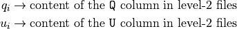
Analytically, Stokes spectra are (possibly weighted) histograms in pulse-invariant space where, given the definition

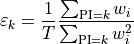
$\varepsilon_k = \frac{1}{T} \frac{\sum_{\text{PI}=k} w_i}{\sum_{\text{PI}=k} w_i^2}$

the content of the k-th bin is given by

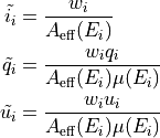
$I_k &= \displaystyle \varepsilon_k \sum_{\text{PI}=k} w_i \quad \text{and} \quad \sigma_{I_k} = \varepsilon_k \sqrt{\sum_{\text{PI}=k} w_i^2}\\ Q_k &= \displaystyle \varepsilon_k \sum_{\text{PI}=k} w_i q_i \quad \text{and} \quad \sigma_{Q_k} = \varepsilon_k \sqrt{\sum_{\text{PI}=k} (w_i q_i)^2}\\ U_k &= \displaystyle \varepsilon_k \sum_{\text{PI}=k} w_i u_i \quad \text{and} \quad \sigma_{U_k} = \varepsilon_k \sqrt{\sum_{\text{PI}=k} (w_i u_i)^2}$

It is worth mentioning that for an un-weighted analysis (i.e., when the weights are unitary for all the events) the above expressions reduce to the more familiar ones

$\displaystyle \varepsilon_k & \xrightarrow[w_i = 1]{} \frac{1}{T}\\ \displaystyle I_k & \xrightarrow[w_i = 1]{} \frac{N_k}{T} \quad \text{and} \quad \sigma_{I_k} \xrightarrow[w_i = 1]{} \frac{\sqrt{N_k}}{T}\\ \displaystyle Q_k & \xrightarrow[w_i = 1]{} \frac{1}{T} \sum_{\text{PI}=k} q_i \quad \text{and} \quad \sigma_{Q_k} \xrightarrow[w_i = 1]{} \frac{1}{T} \sqrt{\sum_{\text{PI}=k} q_i^2}\\ \displaystyle U_k & \xrightarrow[w_i = 1]{} \frac{1}{T} \sum_{\text{PI}=k} u_i \quad \text{and} \quad \sigma_{U_k} \xrightarrow[w_i = 1]{} \frac{1}{T} \sqrt{\sum_{\text{PI}=k} u_i^2}.$

The reader is referred to the section about the XSPEC support for more details about one would use binned Stokes spectra in a spectro-polarimetric fit using XSPEC.

Normalized Stokes spectra¶

xpbin provides facilities to produce normalized Stokes spectra (i.e., spectra where the Q and U channels are divided by the corresponding I channels) with the PHA1QN and PHA1UN binning algorithms:

Q/I, mapped to *pha1qn.fits files via the ixpeobssim.binning.polarization.xEventBinningPHA1QN class;
U/I, mapped to *pha1un.fits files via the ixpeobssim.binning.polarization.xEventBinningPHA1UN class.

This can be used in purely polarimetric fits, e.g., in XSPEC, with the spectral part of the problem completely factored out—more about this in the section about XSPEC support.

Polarization analysis¶

Binned Stokes cubes are not the only binned data product that is relevant to polarization measurement. ixpeobssim provides a series of data structures designed to hold broadband polarization information—possibly in multiple energy layers and sky-coordinate bins.

Warning

One important point to emphasize up-front is that the formalism described in this section neglects by construction the effect of the energy dispersion (which is instead properly handled when fitting with XSPEC). The focus, here, is to provide model-independent quantities that are easy to calculate and visualize, rather than guaranteeing full accuracy.

Whether that is actually important or not depends critically on the application. Comparing the relevant data products binned in true and reconstructed energy (you can toggle the --mc command-line switch to do just that) is a way to gauge the effect of the energy dispersion in a given, particular setup.

Basic formalism¶

All the polarization analysis in ixpeobssim is based on the paper by Kislat et al. (2015), whose formalism is (partially) implemented verbatim (well, almost—you will notice that IXPE adopts a slightly different convention for the event-by-event Stokes parameters, resulting in a factor of 2 popping out here and there) in the ixpeobssim.evt.kislat2015 Python module.

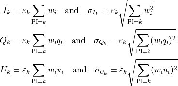
More specifically, for each event we define the three additive reconstructed quantities

$\tilde{i_i} & = \frac{w_i}{A_{\rm eff}(E_i)} \\ \tilde{q_i} & = \frac{w_i q_i}{A_{\rm eff}(E_i)\mu(E_i)} \\ \tilde{u_i} & = \frac{w_i u_i}{A_{\rm eff}(E_i)\mu(E_i)}$

A few remarks on these basic definitions:

the inverse of the effective area in the definition of the weights acts as an acceptance correction guaranteeing that the relevant quantities are summed (or averaged) over the input source spectrum—as opposed to the measured count spectrum;
any additional (multiplicative) event-by-event weight can be easily incorporated into the first term (and gets automatically propagated to the other two);
the effective area and modulation factor are calculated at the measured energy—see the warning above about the effect of the energy dispersion.

(Note the lack of treatment for the energy dispersion is a consequence of our, largely simplistic, implementation of the full formalism described in Kislat et al. (2015), rather than a fundamental limitation of the paper.)

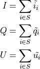
That all said, the measured Stokes parameters over a generic subset S of the events (be that a specific energy range, or a spatial bin in sky coordinates), is obtained by simply summing the event-by-event quantities:

$I & = \sum_{i \in S} \tilde{i_i}\\ Q & = \sum_{i \in S} \tilde{q_i}\\ U & = \sum_{i \in S} \tilde{u_i}$

Warning

This formalism has been thoroughly tested with Monte Carlo simulation, and provides the right answer in the limit of large statistics (i.e., for any sensible polarization analysis). When the statistics is low, though, due to the very nature of the quantities defined above, the recovered Q and U Stokes parameters can lie outside the physical bounds.

Counter-intuitive as it is, this is the same as saying that, with low statistics, you can have an upward fluctuation of the measured modulation and, when you divide by the modulation factor to recover the polarization, there is nothing preventing the latter from exceeding 1.

You should be aware of the limitation of this method when dealing with small samples. The uncertainties on Q and U will tell you right away whether that is the case.

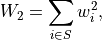
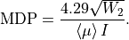
The polarization degree and angle can be recovered with the usual formulae, and Kislat et al. (2015) provides all the facilities to propagate the statistical uncertainties. Note that, in a weighted scheme, the error propagation requires keeping track of the sum of the weights squared

$W_2 = \sum_{i \in S} w^2_i,$

and the minimum detectable polarization reads

$\text{MDP} = \frac{4.29 \sqrt{W_2}}{\left< \mu \right> I }.$

Two related, interesting quantities are the effective number of events and the fractional weight

$N_\text{eff} & = \frac{I^2}{W_2}\\ f_w & = \frac{N_\text{eff}}{N}$

which reduce to the actual number of counts (and to 1, respectrively), in the un-weighted case. Incidentally, these quantities are used to build the effective area in the weighted case.

Warning

The polarization cubes, maps and map cubes are not equipped (yet) to treat the background, or any estimate of the background, in any specific way.

Note

New in version 25.0.0.

All the binned data structures have been largely reworked to add the necessary infrastructure to keep track of the errors on the Stokes parameters and the significance of a detection.

Polarization cubes¶

The simplest possible data structure holding polarization information is a polarization cube. A polarization cube is generated by xpbin run with the --algorithm PCUBE command-line switch, and is stored as a FITS binary table where the relevant metrics are calculated in energy bins.

ixpeobssim.binning.polarization.xBinnedPolarizationCube is the basic read interface to polarization cubes.

The following snippet from the source code should be self-explaining.

class xBinTableHDUPCUBE(xBinTableHDUBase):

    """Binary table for binned PCUBE data.
    """

    NAME = 'POLARIZATION'
    HEADER_KEYWORDS = []
    # Be careful: if you change any of these, make sure you update the
    # MDP_COLUMNS and POL_COLUMNS class members below, as this all need to be
    # in synch with the MDP and polarization maps and map cubes.
    DATA_SPECS = [
        ('ENERG_LO', 'E', 'keV', 'low energy bound'),
        ('ENERG_HI', 'E', 'keV', 'high energy bound'),
        ('E_MEAN'  , 'E', 'keV', 'average energy within the bin'),
        ('COUNTS'  , 'J', ''   , 'number of counts'),
        ('MU'      , 'E', ''   , 'effective modulation factor'),
        ('W2'      , 'E', ''   , 'sum of weights squared'),
        ('N_EFF'   , 'E', ''   , 'effective number of events w/o acceptance correction'),
        ('FRAC_W'  , 'E', ''   , 'N_EFF / COUNTS'),
        ('MDP_99'  , 'E', ''   , 'minimum detectable polarization at the 99% CL'),
        ('I'       , 'E', ''   , 'I Stokes parameter'),
        ('I_ERR'   , 'E', ''   , '1-sigma uncertainty on I'),
        ('Q'       , 'E', ''   , 'Q Stokes parameter'),
        ('Q_ERR'   , 'E', ''   , '1-sigma uncertainty on Q'),
        ('U'       , 'E', ''   , 'U Stokes parameter'),
        ('U_ERR'   , 'E', ''   , '1-sigma uncertainty on U'),
        ('QN'      , 'E', ''   , 'normalized Q Stokes parameter Q/I'),
        ('QN_ERR'  , 'E', ''   , '1-sigma uncertainty on Q/I'),
        ('UN'      , 'E', ''   , 'normalized U Stokes parameter Q/I'),
        ('UN_ERR'  , 'E', ''   , '1-sigma uncertainty on U/I'),
        ('QUN_COV' , 'E', ''   , 'covariance between QN and UN'),
        ('PD'      , 'E', ''   , 'measured polarization degree'),
        ('PD_ERR'  , 'E', ''   , '1-sigma uncertainty on the polarization degree'),
        ('PA'      , 'E', 'deg', 'measured polarization angle'),
        ('PA_ERR'  , 'E', 'deg', '1-sigma uncertainty on the polarization angle'),
        ('P_VALUE' , 'E', ''   , 'p-value for the null hypothesis (no polarization)'),
        ('CONFID'  , 'E', ''   , 'confidence of the polarization detection'),
        ('SIGNIF'  , 'E', ''   , 'detection significance in equivalent gaussian sigma')
        ]
    COL_NAMES = [col_name for col_name, *_ in DATA_SPECS]
    # Be careful: these need to be in synch with the DATA_SPECS above.
    # MDP_COL_NAMES defines the extensions of the MDP maps and map cubes.
    # POL_COL_NAMES defines the extensions of the polarization maps and map cubes.
    MDP_COL_NAMES = COL_NAMES[2:10]
    POL_COL_NAMES = COL_NAMES[2:]

It is worth mentioning that, while some of the columns (i.e., polarization degree and angle, associated uncertainties and MDP) can be calculated from the others (and, are, in fact, recalculated when polarization cubes are summed over the three detector units) we include this redundant information in the FITS file as a convenience.

Polarization-map cubes¶

Polarization-map cubes hold the exact same information as polarization cubes, but binned in sky-coordinates. Each column in a polarization cube maps directly into an image extension in the corresponding polarization-map cube file. Each image extension has three dimensions (two for the spatial binning and one for the energy binning), and the EBOUNDS binary table holds the physical bounds for the energy layers.

Polarization-map cubes are generated by xpbin run with the --algorithm PMAPCUBE command-line switch, and the main read-interface is ixpeobssim.binning.polarization.xBinnedPolarizationMapCube.

Tip

xpbin provides a PMAP binning a mode that is simply an alias for a polarization-map cube with a single energy layer—which we refer to as a polarization map.

MDP-map cubes¶

MDP-map cubes are stripped-down versions of polarization cubes where only the necessary information for the calculation of the minimum detectable polarization is retained.

No.    Name      Ver    Type      Cards   Dimensions   Format
PRIMARY       1 xPrimaryHDU     50   ()
E_MEAN        1 ImageHDU        24   (1, 1, 1)   float64
COUNTS        1 ImageHDU        24   (1, 1, 1)   float64
MU_MDP        1 ImageHDU        24   (1, 1, 1)   float64
I_MDP         1 ImageHDU        24   (1, 1, 1)   float64
W2_MDP        1 ImageHDU        24   (1, 1, 1)   float64
MDP_99        1 ImageHDU        24   (1, 1, 1)   float64
N_EFF         1 ImageHDU        24   (1, 1, 1)   float64
FRAC_W        1 ImageHDU        24   (1, 1, 1)   float64
EBOUNDS       1 xBinTableHDUEBOUNDS     34   1R x 2C   ['E', 'E']

MDP-map cubes are generated by xpbin run with the --algorithm MDPMAPCUBE command-line switch, and the main read-interface is ixpeobssim.binning.polarization.xBinnedMDPMapCube.

Tip

xpbin provides a MDPMAP binning a mode that is simply an alias for a MDP-map cube with a single energy layer—which we refer to as a MDP map.

Livetime-cubes¶

xpbin provides livetime map cubes in sky coordinates and off axis angle bins; livetime-cubes are generated by xpbin run with the --algorithm LTCUBE command-line switch, and the main read-interface is ixpeobssim.binning.exposure.xBinnedLivetimeCube);

Miscellanea¶

xpbin provides additional facilities not strictly related to polarizations—namely:

binned count maps in sky coordinates (use the --algorithm CMAP command-line switch for generation, read interface is ixpeobssim.binning.misc.xBinnedMap);
binned pulse profiles (use the --algorithm PP command-line switch for generation, read interface is ixpeobssim.binning.misc.xBinnedPulseProfile);
binned area-rate maps in detector coordinates (use the --algorithm ARMAP command-line switch for generation, read interface is ixpeobssim.binning.misc.xBinnedAreaRateMap);
binned energy-flux maps in detector coordinates (use the --algorithm EFLUX command-line switch for generation, read interface is ixpeobssim.binning.misc.xBinnedAreaEnergyFluxMap);
binned light curves (use the --algorithm LC command-line switch for generation, read interface is ixpeobssim.binning.misc.xBinnedLightCurve).

Binned data products¶

Stokes spectra¶

Binary table definition¶

Technical details¶

Normalized Stokes spectra¶

Polarization analysis¶

Basic formalism¶

Polarization cubes¶

Polarization-map cubes¶

MDP-map cubes¶

Livetime-cubes¶

Miscellanea¶

Navigation

Related Topics