Event Display
Added in version 29.4.0: ixpeobssim includes a single event display to render the track images shipped with publicly distributed the level-1 files.
As of version 29.4.0 ixpeobssim include a new small application, xpevtdisplay, that allows to display the track images shipped with the standard IXPE level-1 publicily distributed through HEASARC.
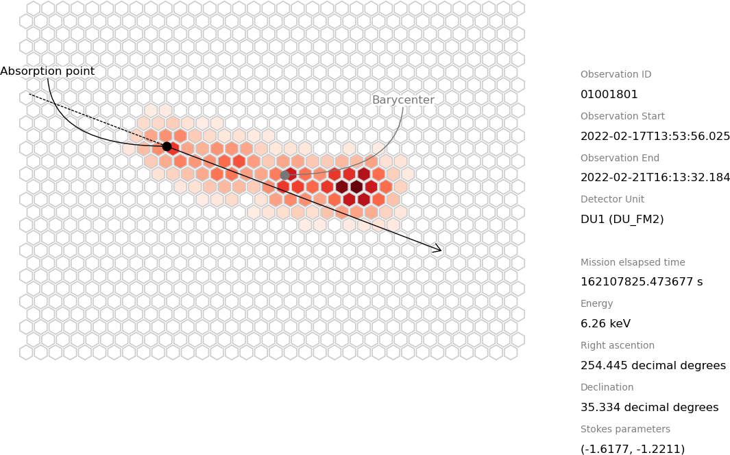
Sample display of a track image—note that mileage may vary depending on the setting (i.e., command-line switches) used in xpevtdisplay.
While the help coming with the program should be largely self-explaining, a few remarks are in order, here. First of all, xpevtdisplay operates on level-1 files, which are the only ones containing the track images by default, and whom most user are probably not terribly familiar with. In constrast to the more widely used level-2 files, level-1 files are significantly larger (which means: do not be surprised if firing up the event display on a particular file takes a few seconds), and contain all the event recorded through the observation—no matter whether they correspond to actual GTI, or to periods when the source was occulted by the Earth (and, possibly, with one of the calibration sources in use). As a consequence, just firing up the event display on a level-1 file
xpevtdisplay path_to_my_level1_file
is not terribly useful, in general: you have no control on which events you are actually displaying—that is, they might very well be from one of the onboard calibration sources, rather than from the celestial source being observed.
For this very reason, xpevtdisplay features a --evtlist command
line flag that allows to feed into the application a level-2 file in addition
to the level-1 main file (it goes without saying, the two generally need to
correspond to the same observation).
xpevtdisplay path_to_my_level1_file --evtlist path_to_the_fellow_level2_file
When you pass this additional file to the event display, a few things happen behind the scenes, namely:
the display will loop over the level-2 file, one event at a time, and retrieve all the relevant high-level information (time, energy, sky position and Stokes parameters);
for each event, a binary search is run over the level-1 file to identify the corresponding raw event data;
the actual event in the level-1 file gets displayed, along with all the high-level info from the level-2 data.
This is where things get interesting: since you can run xpeselect natively over any level-2 file, this provides a convenient mechanism to select small subsamples of event (e.g., in energy or sky position) and get them displayed.
Now, when you start looking at track images, you will probably get bored
quite quickly: as the IXPE effective area is sharply peaked around 2.2 keV,
most of the events will probably look quite similar to each other. This is fine
if you are interested in an unbiased sample of tracks, but it will take you lots
of luck to stumble across a high-energy track such as the one shown at the top
of the page. For this reason, the --resample command-line swicht provides
a mechanism to resample in energy the input level-2 file using a power law with
the specified index—if you use, e.g., --resample 3 you should see a large
variety of event topologies.
Warning
Be mindful that, since the event time is the only quantity that we can use to keep in synch level-2 and level-1 data, the event list functionality does not play well with any analysis tool (e.g., the barycorr FTOOL) that change the event time—for the purpose of the event display you want to use event file as distributed, without further processing.
Also, when reading a Level-1 files and passing at the same time an event list in the form of a Level-2 file, you should make sure that the former covers the entire time span of the latter, otherwise the MET bisection will fail. If the Level-2 file covers a longer time span wrt. the Level-1 file, you can simply trim the former with the standard tools.
Observation animations
Building on top of the single event display, ixpeobssim provides a separate application, xpobsdisplay, that allows to create complex animations starting from the standard observation products distributed through HEASARC by jut adding to the track images accumulating histograms of the relevant science quantities: energy, sky position, and Stokes parameters.
The xpobsdisplay is fairly similar to that of xpevtdisplay. We won’t describe the meaning of all the command-line switches here, but the following command
xpobsdisplay path_to_my_level1_file --evtlist path_to_the_fellow_level2_file \
    --resample 2 --autostop 200 --targetname "The name of the source" --autosave True \
    --imgdpi 200 --batch True
will read in the target files and write to file 200 still track images in batch mode (i.e., no matplotlib canvas will be displayed on the screen).
The user can then combine the still frames into an actual animation by using any of the countless tools available on the market, one possible example being
ffmpeg -framerate 1 -i path_to_frames_%04d.png -c:v libx264  -s 1920x1080 -r 30 \
    -pix_fmt yuv420p animation.mp4
For completeness, a succinct and yet informative resource about using ffmpeg to create slideshows is here.