Toy source models
Toy source models are a great way to get acquainted with the internals of ixpeobssim and learn how to build physically meaningful models. Below is a short gallery of simple models illustrating the basic functionalities of ixpeobssim.
Single point source
Source file: [github]/ixpeobssim/config/toy_point_source.py
Simulation/analysis pipeline: [github]/ixpeobssim/examples/toy_point_source.py
import numpy

from ixpeobssim.config import file_path_to_model_name
from ixpeobssim.utils.matplotlib_ import plt, setup_gca
from ixpeobssim.srcmodel.roi import xPointSource, xROIModel
from ixpeobssim.srcmodel.spectrum import power_law
from ixpeobssim.srcmodel.polarization import constant
from ixpeobssim.utils.fmtaxis import fmtaxis


__model__ = file_path_to_model_name(__file__)
ra, dec = 30., 45.
pl_norm = 10.
pl_index = 2.
spec = power_law(pl_norm, pl_index)
pd = 0.1
pa = 30.
pol_deg = constant(pd)
pol_ang = constant(numpy.radians(pa))

src = xPointSource('Point source', ra, dec, spec, pol_deg, pol_ang)

ROI_MODEL = xROIModel(ra, dec, src)
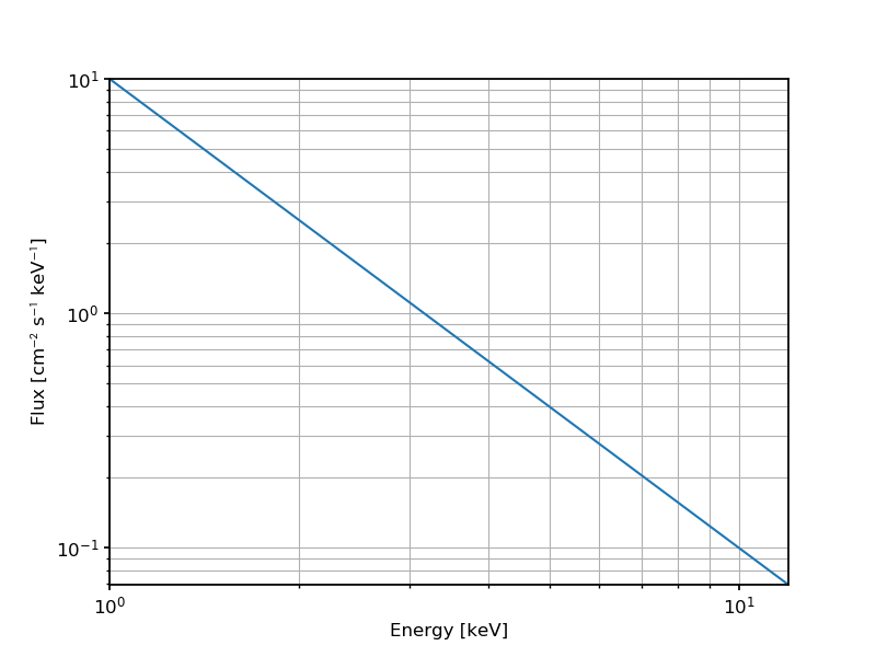
This is possibly the simplest interesting model that can be simulated: a point source with a time-independent power-law spectrum and time- and energy-independent polarization degree and angle.
The only meaningful feature of the source that can be plotted is its energy spectrum, which is shown below.
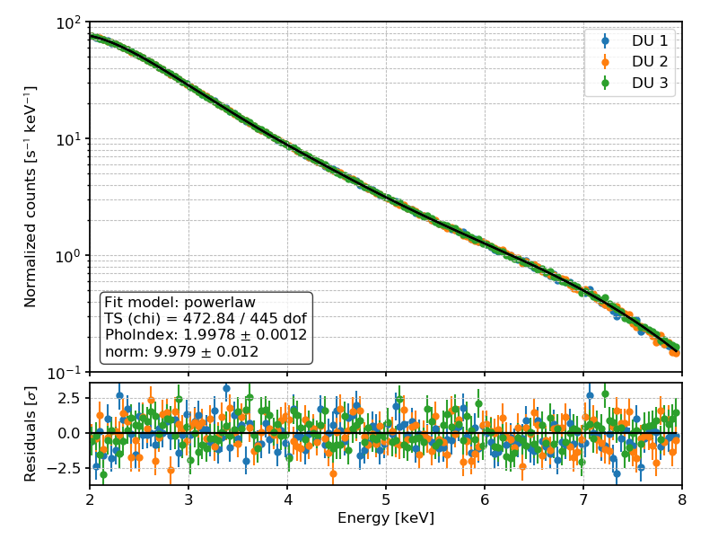
And here is a spectral fit with XSPEC to a set of event lists created with xpobssim and binned with xpbin:
Two point sources
Source file: [github]/ixpeobssim/config/toy_mutiple_sources.py
Simulation/analysis pipeline: [github]/ixpeobssim/examples/toy_mutiple_sources.py
import numpy

from ixpeobssim.config import file_path_to_model_name
from ixpeobssim.utils.matplotlib_ import plt, setup_gca
from ixpeobssim.srcmodel.roi import xPointSource, xROIModel
from ixpeobssim.srcmodel.spectrum import power_law
from ixpeobssim.srcmodel.polarization import constant
from ixpeobssim.utils.units_ import arcmin_to_degrees
from ixpeobssim.utils.fmtaxis import fmtaxis


__model__ = file_path_to_model_name(__file__)
ra, dec = 30., 45.

ra1, dec1 = ra, dec
pl_norm1 = 1.
pl_index1 = 2.
spec1 = power_law(pl_norm1, pl_index1)
pol_deg1 = constant(0.25)
pol_ang1 = constant(numpy.radians(30.))

ra2, dec2 = ra + arcmin_to_degrees(2.), dec - arcmin_to_degrees(3.)
pl_norm2 = 0.25
pl_index2 = 1.5
spec2 = power_law(pl_norm2, pl_index2)
pol_deg2 = constant(0.)
pol_ang2 = constant(numpy.radians(0.))

src1 = xPointSource('Point source 1', ra1, dec1, spec1, pol_deg1, pol_ang1)
src2 = xPointSource('Point source 2', ra2, dec2, spec2, pol_deg2, pol_ang2)

ROI_MODEL = xROIModel(ra, dec, src1, src2)
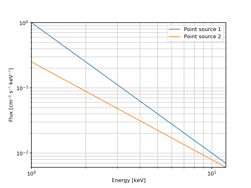
This is a slight variation over the single point source, where we include in the same region of interest two stationary point sources, with different power-law spectra and polarization patterns, offset by a few arcminutes with respect to the center of the ROI.
For completeness, below are the energy spectra for the two sources.
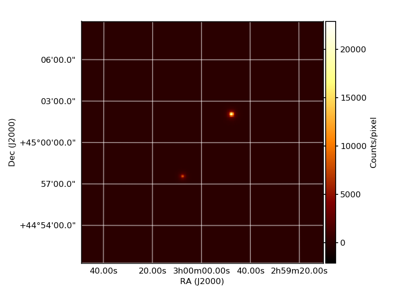
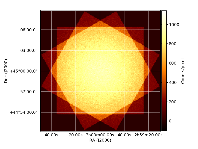
And here is a count map created from a simulated observation of this ROI model using xpbin in CMAP mode.
Tip
In this case we are using the ability of ixpeobssim to overlay multiple
sources in the same ROI to simulate two physically distinct objects, but
subclasses of ixpeobssim.srcmodel.roi.xModelComponentBase should
in fact be thought of as model components, and this is the very same
technique that we use to simulate different physical components of the same
object.
Uniform disk
Source file: [github]/ixpeobssim/config/toy_disk.py
Simulation/analysis pipeline: [github]/ixpeobssim/examples/toy_disk.py
import numpy

from ixpeobssim.config import file_path_to_model_name
from ixpeobssim.utils.matplotlib_ import plt, setup_gca
from ixpeobssim.srcmodel.roi import xUniformDisk, xROIModel
from ixpeobssim.srcmodel.spectrum import power_law
from ixpeobssim.srcmodel.polarization import constant
from ixpeobssim.utils.units_ import arcmin_to_degrees
from ixpeobssim.utils.fmtaxis import fmtaxis


__model__ = file_path_to_model_name(__file__)
ra, dec = 45., 45.
radius = arcmin_to_degrees(10.)
pl_norm = 1.
pl_index = 2.
spec = power_law(pl_norm, pl_index)
pol_deg = constant(0.5)
pol_ang = constant(numpy.radians(65.))

src = xUniformDisk('Uniform disk', ra, dec, radius, spec, pol_deg, pol_ang)

ROI_MODEL = xROIModel(ra, dec, src)
This is an extended source with the morphology of a uniform disk and a simple power-law spectrum.
The most interesting feature of this toy model is possibly the fact that the disk is larger than the field of view and therefore, if one runs a long-enough simulation and creates a binned map out of the event file, the vignetting of the optics and the footprint of the three focal-plane detector units become evident.
Gaussian disk
Source file: [github]/ixpeobssim/config/toy_gauss_disk.py
Simulation/analysis pipeline: [github]/ixpeobssim/examples/toy_gauss_disk.py
import numpy

from ixpeobssim.config import file_path_to_model_name
from ixpeobssim.utils.matplotlib_ import plt, setup_gca
from ixpeobssim.srcmodel.roi import xGaussianDisk, xROIModel
from ixpeobssim.srcmodel.spectrum import power_law
from ixpeobssim.srcmodel.polarization import constant
from ixpeobssim.utils.units_ import arcmin_to_degrees
from ixpeobssim.utils.fmtaxis import fmtaxis


__model__ = file_path_to_model_name(__file__)
ra, dec = 45., 45.
radius = arcmin_to_degrees(2.)
pl_norm = 1.
pl_index = 2.
spec = power_law(pl_norm, pl_index)
pol_deg = constant(0.5)
pol_ang = constant(numpy.radians(65.))

src = xGaussianDisk('Gaussian disk', ra, dec, radius, spec, pol_deg, pol_ang)

ROI_MODEL = xROIModel(ra, dec, src)
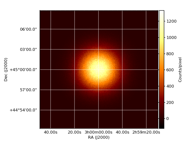
This is very similar to the uniform disk example, except that the morpholgy of the source is a bivariate gaussian (with a diagonal covariance matrix) and the source does not extend as much across the field of view, so that it is pretty much completely contained.
Below is yet another binned coount map from xpbin in CMAP mode.
A periodic source
Source file: [github]/ixpeobssim/config/toy_periodic_source.py
Simulation/analysis pipeline: [github]/ixpeobssim/examples/toy_periodic_source.py
import numpy

from ixpeobssim.config import file_path_to_model_name
from ixpeobssim.utils.matplotlib_ import plt, setup_gca
from ixpeobssim.srcmodel.roi import xPeriodicPointSource, xROIModel
from ixpeobssim.srcmodel.ephemeris import xEphemeris
from ixpeobssim.srcmodel.spectrum import power_law
from ixpeobssim.srcmodel.polarization import constant
from ixpeobssim.utils.fmtaxis import fmtaxis
from ixpeobssim.utils.time_ import string_to_met_utc


__model__ = file_path_to_model_name(__file__)
ra, dec = 45., 45.

def pl_norm(phase):
    """Energy spectrum: power-law normalization as a function of the pulse
    phase.
    """
    return 2. * (1.25 + numpy.cos(4 * numpy.pi * phase))

pl_index = 2.
spec = power_law(pl_norm, pl_index)

def pol_deg(E, phase, ra=None, dec=None):
    """Polarization degree as a function of the dynamical variables.

    Since we're dealing with a point source the sky direction (ra, dec) is
    irrelevant and, as they are not used, defaulting the corresponding arguments
    to None allows to call the function passing the energy and phase only.
    """
    norm = numpy.clip(E / 10., 0., 1.)
    return norm * (0.5 + 0.25 * numpy.cos(4 * numpy.pi * (phase - 0.25)))

pol_ang = constant(numpy.radians(65.))

start_date = '2022-04-21'
t0 = string_to_met_utc(start_date, lazy=True)
nu0 = 0.1363729749
nudot0 = 0.543638e-13
ephemeris = xEphemeris(t0, nu0, nudot0)
src = xPeriodicPointSource('Periodic source', ra, dec, spec, pol_deg, pol_ang, ephemeris)

ROI_MODEL = xROIModel(ra, dec, src)
This is a fairly complicated toy example, illustrating a number of ixpeobssim features.
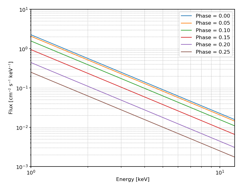
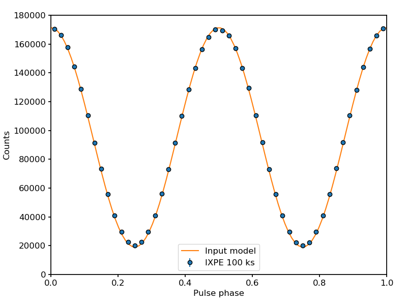
The ROI includes a single point source with a power-law spectrum, but this time around, the source being periodic, the corresponding power-law normalization varies with the pulse phase according to a simple analytical formula. (In order to make the comparison of the simulation output with the input model straightforward the power-law index is constant.) Below is the normalization as a function of the pulse phase

along with the actual differential energy spectrum, plotted at several different pulse phases.
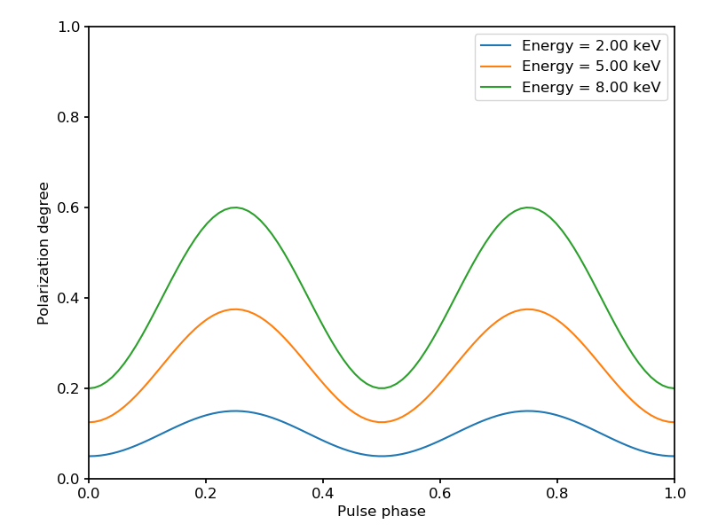
The polarization angle is constant, but for illustration purposes the polarization degree varies with the pulse phase according to yet another simple formula, as shown in the plot below:
Here is an example of a binned pulse profile from an event list produced by ixpeobssim, compared with the input model.
And below is an example of a slightly more complicated analysis, where we
fold the original event list with the ephemeris of the input model;
split the original even list into a number of phase bins;
estimate the polarization degree into two energy bins (within each phase bin) and compare with the input model.
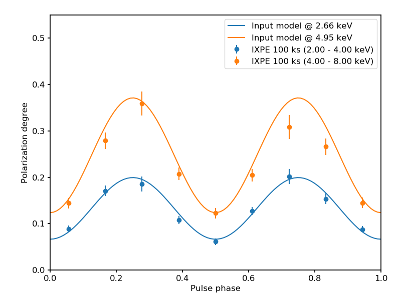
For completeness, the polarization degree is evaluated by summing the event-by-event Stokes parameters, i.e., without taking into account the energy redstribution—which is probably account for most of the slight bias that can be see in the plot. The input model is evaluated at the average photon energy within each bin.
A model from XSPEC
Source file: [github]/ixpeobssim/config/toy_xspec_point_source.py
Simulation/analysis pipeline: [github]/ixpeobssim/examples/toy_xspec_point_source.py
import numpy

from ixpeobssim.config import file_path_to_model_name
from ixpeobssim.utils.matplotlib_ import plt, setup_gca
from ixpeobssim.srcmodel.roi import xPointSource, xROIModel
from ixpeobssim.srcmodel.polarization import constant
from ixpeobssim.srcmodel.spectrum import xXspecModel


__model__ = file_path_to_model_name(__file__)
ra, dec = 45., 45.
# Parameters for a complex XSPEC spectral model phabs*(bbody+powerlaw)
expression = 'phabs * (bbody + powerlaw)'
col_dens = 1.
bb_temp = 1. #in keV
# bb_norm is the luminosity in units of 1e39 erg/s over
# the distance squared in units of 10 kpc
bb_norm = 1e-3 / (0.1**2)
pl_index = 2.
pl_norm = 10.

spec = xXspecModel(expression, [col_dens, bb_temp, bb_norm, pl_index, pl_norm])
pd = 0.5
pa = 30.
pol_deg = constant(pd)
pol_ang = constant(numpy.radians(pa))

src = xPointSource('Point source', ra, dec, spec, pol_deg, pol_ang)

ROI_MODEL = xROIModel(ra, dec, src)