Showcase
NGC 1068
Source file: [github]/ixpeobssim/config/ngc1068.py
Simulation/analysis pipeline: [github]/ixpeobssim/examples/ngc1068.py
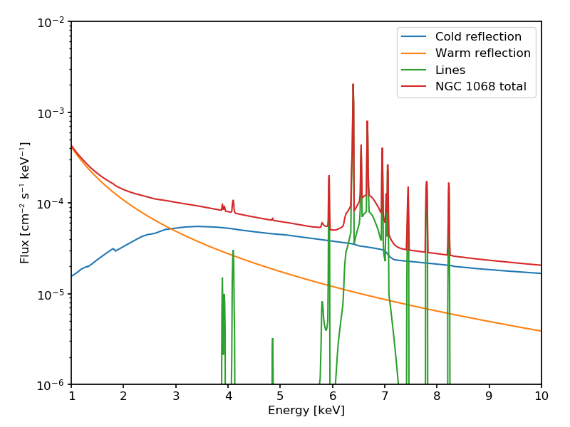
This is an example of a spectro-polarimetric model of a Compton-thick AGN, and a well-known one, where we have detailed information about the source geometry and energy spectrum.
There are three distinct spectral components to the model, each one with its own polarimetric pattern:
the cold reflection from the torus;
the warm reflection from the cone;
the emission lines.
As far as the geometry for the polarimetric modeling is concerned, the ionization cone is assumed to be perpendicular to the plane of the torus, and the inclination angle of the system is 75 degrees.
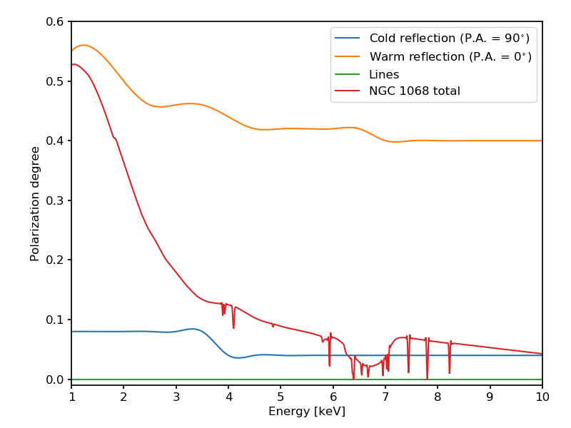
We note that the position angles for the cold and warm relflection components are orthogonal to each other, so that this source is a good illustration of the harmonic addition in ixpeobssim.
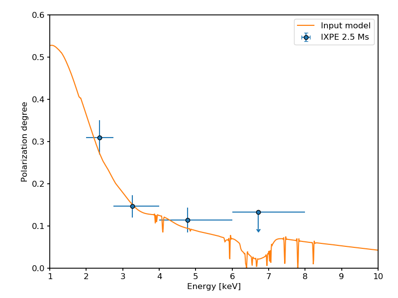
Simulation output
Below is an output of an ixpeobssim simulation, where the measured polarization degree, estimated in a few energy bins, is compared to the input model.
References
[1] Ghisellini, G.; Haardt, F.; Matt, G., “The Contribution of the Obscuring Torus to the X-Ray Spectrum of Seyfert Galaxies - a Test for the Unification Model”, Monthly Notices of the Royal Astronomical Society, Vol. 267, NO. 3/APR1, P. 743, 1994
[2] Goosmann, R. W.; Matt, G., “Modeling X-ray polarimetry while flying around the misaligned outflow of NGC 1068”, SF2A-2011: Proceedings of the Annual meeting of the French Society of Astronomy and Astrophysics, 2011
#Crab pulsar #———– # #* Source file: [github]/ixpeobssim/config/crab_pulsar.py #* Simulation/analysis pipeline: [github]/ixpeobssim/examples/crab_pulsar.py # #.. automodule:: ixpeobssim.config.crab_pulsar
Cas A
Full source model definition can be found in ixpeobssim.config.toy_casa.py.
The spectral model is taken from E.A. Helder and J. Vink, “Characterizing the non-thermal emission of Cas A”, Astrophys.J. 686 (2008) 1094–1102, http://arxiv.org/abs/0806.3748. The spectrum of Cas A is a complex superposition of thermal and non thermal emission, and for our purposes, we call thermal anything that is making up for the lines and non-thermal all the rest.
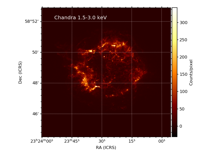
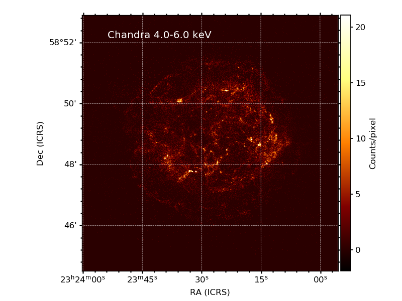
We have two images of Cas A, at low (1.5–3.0 keV) and high (4.0–6.0 keV) and, due to the absence of lines between 4 and 6 keV we’re attaching the latter to the non-thermal spectrum and the former to the thermal component.
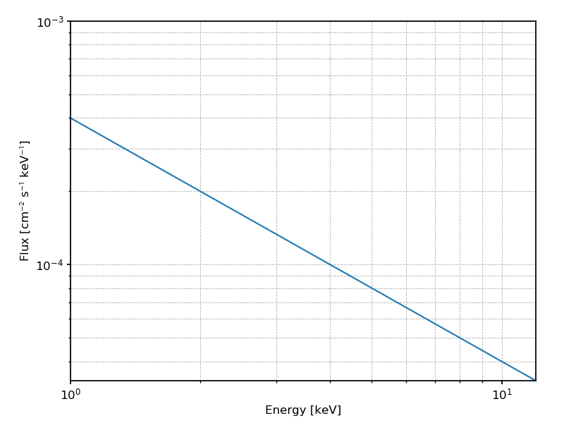
Here is the photon spectrum we are using for the simulation of Cas A:
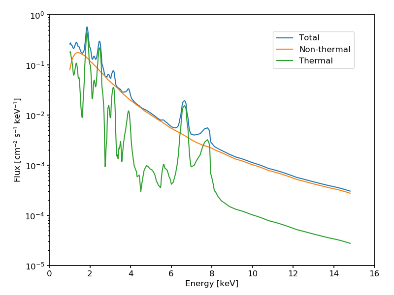
The morphology of the source is energy-dependent in a non trivial way. We start from two Chandra images (in the 1.5–3 keV and 4–6 keV energy ranges, respectively) and associate the former to the thermal spectral component and the latter to the non-thermal one (note the absence of spectral lines between 4 and 6 keV).
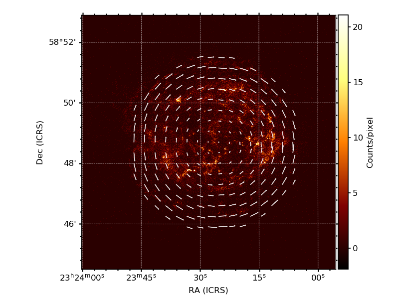
For the polarization, we assume that the thermal component is unpolarized, while for the non-thermal component we use a simple geometrical, radially symmetric model (loosely inspired from radio observations) where the polarization angle is tangential and the polarization degree is zero at the center of the source and increases toward the edges reaching about 50% on the outer rim of the source (see figure below).
Our total model of the region of interest is therefore the superposition of two indipendent components, with different spectral, morphological and polarimetric properties. Crude as it is, it’s a good benchmark for the observation simulator.
Simulation output
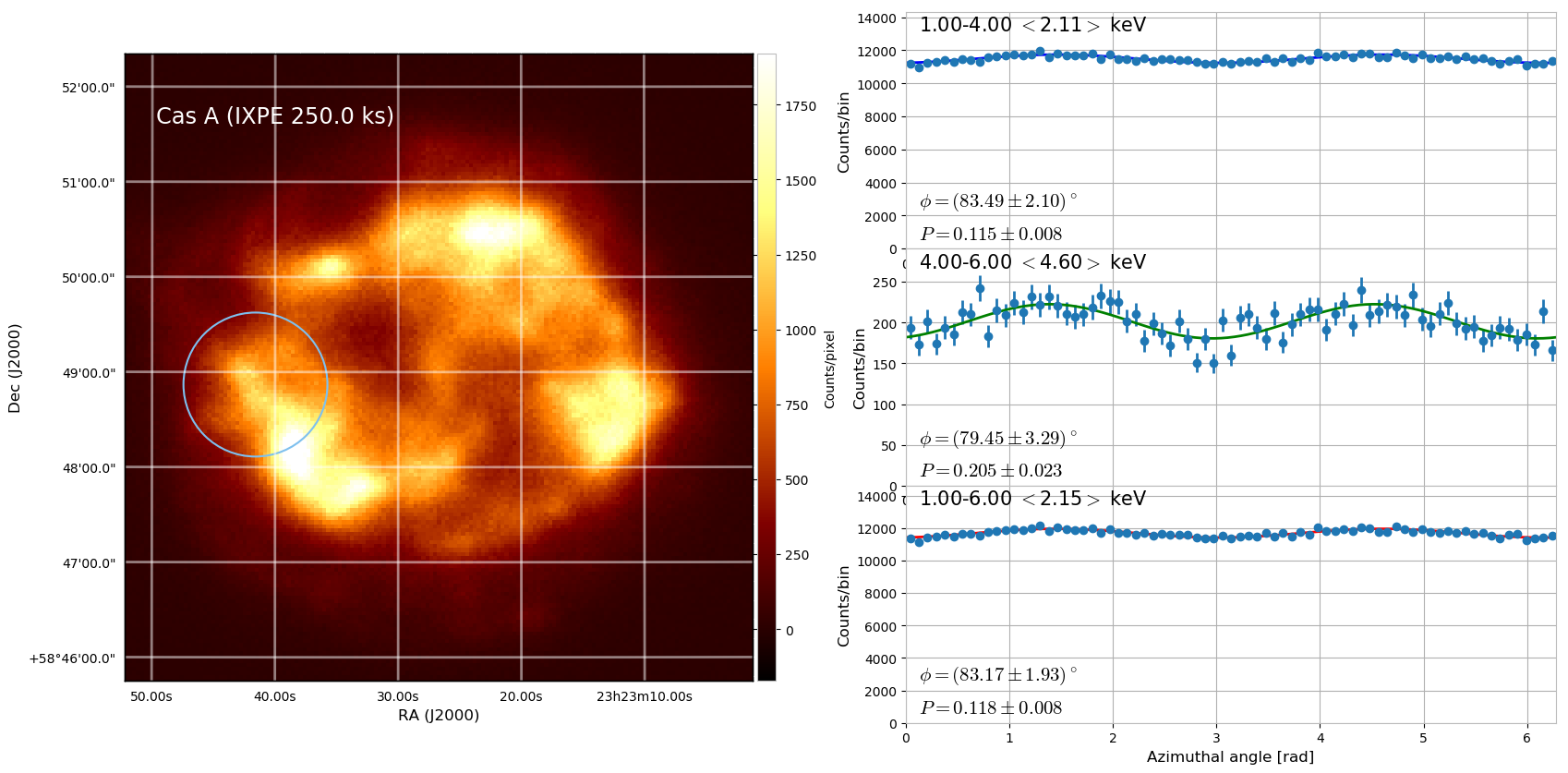
Below is a binned count map of a 250 ks simulated IXPE observation of Cas A, based on the model described above. When the entire source is analyzed at once, most of the polarization averages out and even in the high-energy band, where the emission is predominantly non-thermal, the residual polarization degree resulting from the averaging of the different emission regions is of the order of 5%.

On the other hand, spatially- and energy-resolved polarimetry would in this case reveal much of the richness in the original polarization pattern. Below is an example of the azimuthal distributions in the two energy bands for the circular region of interest indicated by the white circle in the left plot. For reference, the corresponding flux integrated in the region is about 3.5% of that of the entire source. The comparison with the previous, spatially averaged distributions is striking.
By mapping the entire field of view with suitable regions of interest we can in fact (at least qualitatively) recover the input polarization pattern.
Cen A
Source file: [github]/ixpeobssim/config/cena.py
Simulation/analysis pipeline: [github]/ixpeobssim/examples/cena.py
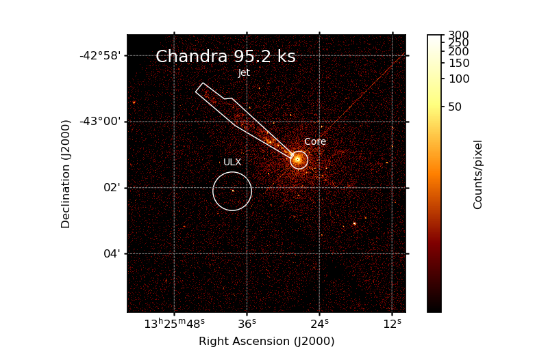
Here we illustrate an example of how to convert a Chandra observation using the xpobssim tool. The simulation concerns the Centaurus A source, based on a Chandra event file taken from the Chandra database (for reference the observation id is 8489). With the xpobssim tool you can also define regions within the ROI using regions. In this example we defined the jet and core regions and the ULX star as can be seen in the figure below.
Simulation output
The plot below refers to a 1.5 Ms simulation. We selected the same three regions to perform spatially resolved polarimetry, marked in the figure below:
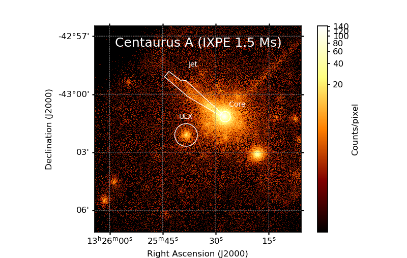
For each of these regions we calculated the MDP value. In this simulation we have also included the instrumental background and when calculating the MDP we take these photons as the background. The results are resumed in following snippet.
Jet region:
2.00--8.00 keV: 12487 src counts (99.5%) in 1.5 Ms, MDP 11.13%
Core:
2.00--8.00 keV: 25844 src counts (100.0%) in 1.5 Ms, MDP 6.46%
ULX:
2.00--8.00 keV: 4370 src counts (99.2%) in 1.5 Ms, MDP 19.24%
Instrumental background
The various incarnations of the instrumental background are peculiar among source components in that the simulation happens in detector (as opposed to sky) coordinates, and the resulting event list is not convolved with any of the instrument response function.
The instrumental background is implemented as an instance of the
ixpeobssim.srcmodel.bkg.xInstrumentalBkg class, or any of its
subclasses. At simulation time, the object effectively produces a uniform,
non-polarized source in the GPD reference frame.
Source file: [github]/ixpeobssim/config/instrumental_bkg.py
Simulation/analysis pipeline: [github]/ixpeobssim/examples/instrumental_bkg.py
This is the simplest possible realization of the instrumental background, where the energy spectrum is a power law fitted to the data from Bunner et al. (1978ApJ…220..261B). Here the authors provide the non X-ray background rates for their three detectors and we are using values for the Neon-filled detector in Table 3 of the paper.
For completeness: this model component can be imported in any ixpeobssim configuration file by simply adding the following line:
from ixpeobssim.config.instrumental_bkg import bkg
Then all you need to do is to add the bkg source to your region of interest.
Warning
Care must be taken in interpreting the output of instrumental background simulations. While the original distribution is flat in detector coordinates, when the photons are looked at in sky coordinates the dithering of the observatory, if enabled, will produce a smearing at the edges of the field of view. In addition, since the default photon spectrum is fairly hard, the energy dispersion can cause noticeable deviations from the input power law.