Orbit, SAA and GTIs
ixpeobssim includes a simplified representation of the IXPE orbit. This allows to calculate the SAA epochs, the target occultation and, ultimately, the good time intervals, in a realistic fashion. While many of these capabilities are similar to those done by the Science Operations Center (SOC) for mission planning, we caution that these capabilities in no way supersede or replace those done by the SOC. They are primarily designed to help account for observational realities when simulating event lists.
Baseline orbit
IXPE was launched on December 9, 2021, in an orbit characterized by:
altitude: 601.1 km
inclination: 0.23 decimal degrees
eccentricity: 0.0012
For the purpose of ixpeobssim simulation we dynamically generate a
TLE matching the
official TLE retrieved right after launch
IXPE
1 49954U 21121A   21351.00640149  .00001120  00000-0  35770-4 0  9994
2 49954   0.2300 281.7657 0011347 134.4260 303.9164 14.90740926  1166
While we are aware that this TLE will no be valid for the lifetime of the IXPE mission, this approximation was tentatively deemed sufficient for the purpose of simulation observations. (In general we don’t aim at getting the actual GTI for a real observation, just realistic ones.) For completeness, we use the skyfield Python package to deal with all the aspects discussed in this section, and the user is referred to the package documentation for more background information.
Note
The nominal mean motion of 14.9 revolutions per day (at an altitude of 600 km) corresponds to a period of 5800 s. Along with the duration of the SAA epochs (810 s on average), this is one of the two fundamental timescales for IXPE observations.
(For completeness, due to the rotation of the Earth, the average time distance between two consecutive SAA entries is 6210 s.)
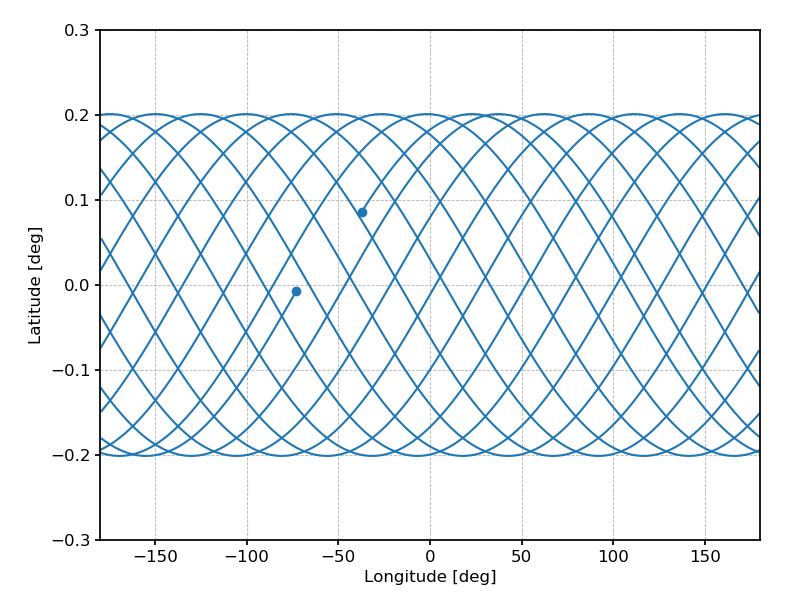
Footprint of the IXPE orbit over the Earth surface for one day of observations.
The South Atlantic Anomaly
We parametrize the South Atlantic Anomaly (SAA) as a 12-vertex convex polygon in Earth coordinates. The initial definition of the polygon is based on the heritage of other observatories (e.g., Fermi LAT and GBM, AGILE) and may be refined after launch, but it is more than adequate for pre-launch simulations.
Note
During the SAA passages in nominal science operations we will lower the high voltage for the focal-plane detectors and we shall not acquire science data. It follows that the SAA is one of the fundamental ingredients for determining the good time intervals for the observation.
IXPE being in nearly-equatorial orbits, the duration of the SAA epochs is approximately the same at each passage, the overall variations being of the order of a few %.
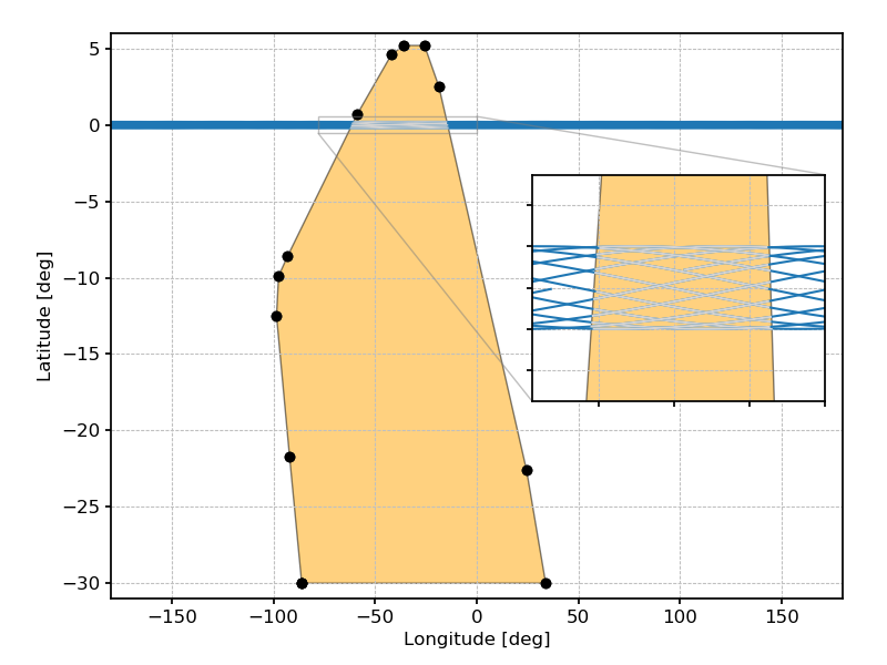
Footprint of the IXPE orbit over the Earth surface for one day of observation, including the SAA polygon. The shaded parts of the satellite track corresponds to the period of times spent inside the SAA, where the observatory does not take data.
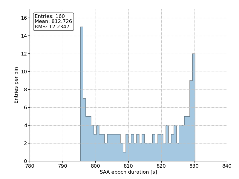
Distribution of the duration of the SAA epochs over 161 consecutive passages.
Note
With an average SAA epoch duration of 813 s every 6213 s, the average fraction of time spent by IXPE in the SAA is about 13%.
Earth Occultation
A simple consideration of the IXPE orbit geometry (a 600 km altitude orbit above a planet with a radius of 6300 km) makes it clear that a large fraction of the sky will be obstructed by the Earth. Just as the SOC is using in the planning stages of the mission, we assume that a particular sky position is occulted by the Earth whenever the minimum altitude of the line of sight is less than 200 km.
A baseline expectation and rule of thumb for observers is that any particular target with declinations in the range of -50 to 50 degrees will be occulted by the Earth for approximately 40% of an orbit. Sources in the declination range of 50-70 degrees experience less time in occultation, and is effectively negligible for sources beyond +/- 70 degrees declination.
For a given target, the fraction of the orbit where the target is occulted by the Earth can be safely treated as a constant value on both short time scales (days or weeks) as well as longer time scales (months or years). No position on the sky should have particular “window of visibilty” where it is observable for unusually long periods of time.
We finally caution that this calculation in particular does not account for some of the expected higher-order effects that will impact the GTI fraction. As an example, the oblateness of the Earth (which will affect the visibility of a target in particular directions) is not modeled here. Tests against the SOC’s tools show that these corrections may affect the total amount of time on-source at about the 1 percent level. Using the target 3C273 as one test case, we found that the SOC predicts this source is visible for 60.0275 percent of the orbit while the calculations included here predict that 3C273 is visible 60.934 percent.
Sun Pitch Angle
Another observational constraint implemented in ixpeobssim is the times of year where a particular target source right ascension and declination is properly separated from the Sun. We currently set the default separations (hereafter the Sun pitch angle) to reside between 65 and 115 degrees. These restrictions will not affect the GTI’s directly (as the Sun pitch angle does not vary significantly over the course of a day or week long exposure) but may help motivate a more sensible choice of start date or help with scheduling a larger number of targets. As stated above, these calculations should only be treated as approximations for the observation planning tools utilized and/or provided by the SOC.
Good time intervals
The wall-clock time of the observation in xpobssim is controlled by four command-line parameters:
startdate: the start date of the observation (default: “2022-04-21”), assumed to be in UTC. This is a string in the%Y-%m-%d(if you don’t care about the precise hour of the day) or%Y-%m-%dT%H:%M:%S.%f(if you do) format;duration: the physical duration of the observation in s;saa: flag instructing xpobssim to consider (i.e., exclude) the SAA passages when calculating the good time intervals (default: False);occult: flag instructing xpobssim to consider (i.e., exclude) the time interval when the target is occulted by the Earth when calculating the good time intervals (default: False)
Since version 8.6.0 xpobssim is equipped to properly take into account the SAA
and the Earth occultation in the calculation of the good time intervals, although
it does not do that by default (i.e., you have to enable the two corresponding
command-line switches for that to happen). Note that, if you run with the
saa and occult flags enabled, your effective on time will be roughly
55% of the physical duration (this is what will happen in real life).
Warning
In a future ixpeobssim version the saa and occult flags will be
enabled by default. In the meantime, any test of the new functionality is
welcome.
Source visibility
When dealing with sensitivity studies, most of the times one is concerned with the total source ontime (i.e., the sum of all good time intervals) rather that the wall-clock duration of the observation, given that the latter has to be accommodated in the context of the overall observing plan. The combined impact of the SAA and Earth occultation will reduce the good time intervals to 53–87% of the total duration of the observation, with the particular value depending almost exclusively on the declination of the source position. Running simulations with all the physical effects (including the SAA passages and Earth occultations) enabled is instructive for estimating the amount of net exposure for a given observation.
In order to help the users planning an observation, and with all the caveats
above, as of version 8.6.0 ixpeobssim provides a rough visibility tool
(xpvisibility.py) summarizing the relevant information, as illustrated in
the figure below.
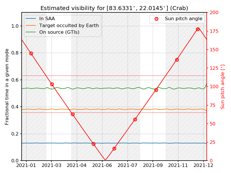
Output of the xpvisibility.py tool, run on the Crab nebula for a
time span of a year starting on January 1, 2021.
For reference, the output of
xpvisibility.py --srcname Crab --startdate 2021-01-01
includes some basic statistics about the duration of the observation, the total sum of good-time internals and the periods when the source is observable due to time constraints.
>>> Target coordinates: R. A. 83.633083, Dec. 22.014500
>>> Start MET for the observation: 126230400.000 s
>>> Stop MET for the observation: 157788000.000 s
>>> Wall-clock duration of the observation: 31557.600 ks
>>> Total GTI: 16959.307 ks (53.7 %)
>>> Average visibility efficiency: 61.827%
>>> Viewing periods (due to Sun constraints):
>>> [01] 2021-02-17T19:53:11.046608--2021-04-09T00:41:20.692787
>>> [02] 2021-08-22T06:13:02.833588--2021-10-12T12:26:04.468925
This can be compared with the output of the HEASARC Viewing Tool
Viewing Results
Input equatorial coordinates:
Crab, resolved by SIMBAD (local cache) to
[ 83.6331°, 22.0145° ], equinox J2000.0

IXPE (planning)

This mission is in the planning stage.

*** VIEWING Version 3.4      run on 2020 May 13 ***
for the period 2020 May 13 to 2022 May 14

With IXPE (Sun angle range =  65-115):
Observable between 2020 Aug 22           and 2020 Oct 12
Observable between 2021 Feb 17           and 2021 Apr 09
Observable between 2021 Aug 22           and 2021 Oct 12
Observable between 2022 Feb 18           and 2022 Apr 09
Dithering
In nominal data-taking configuration the IXPE observatory is dithered around the pointing direction, the main reason for that being averaging out the spurious modulation and making correcting for that practically possible.
The dithering pattern has the basic form
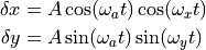
with a default amplitude of 1.6 arcsec and the three periods corresponding to the angular pulsations in a, x and y being 907 s, 101 s and 449 s, respectively.
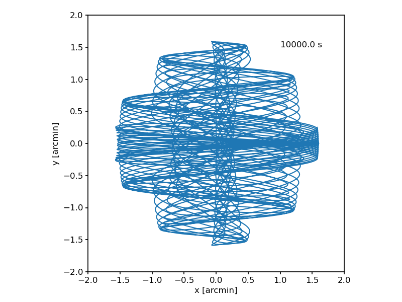
Representation of the default IXPE dithering path for a 10 ks observation.
When convolved with the PSF of the instrument, the dithering pattern provides a image on the focal plane that is approximately uniform (within a factor of 2) for a point source.
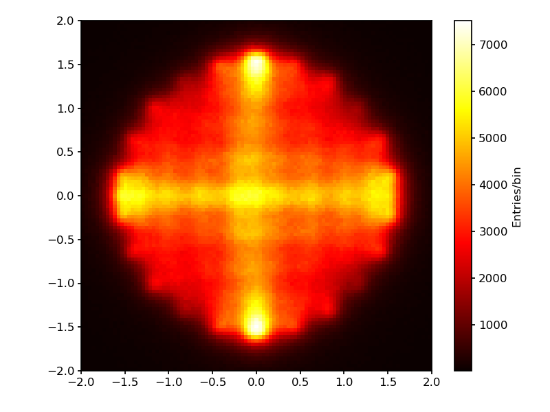
Representation of the dithered image of a point source on the IXPE focal plane.
Pointing history
The pointing history is written in a dedicated extension of the IXPE photon lists
called SC_DATA, with the exact structure described in the section about
Data format.
The pointing history is written at regular time intervals, and the time step can
be set from command line. Tests show that a 10 s interval provides a maximum
error of 0.15 arcsec in the pointing direction in the sky, when the latter is
reconstructed via an interpolated spline from the SC_DATA table. A 5 s time
interval provides a sub-arcsec error in the reconstructed pointing direction.