XSPEC support
Since version 2.4.0 ixpeobssim has a limited support for spectro-polarimetric fitting in XSPEC (thanks to Keith Arnaud). This has been somewhat evolving with time and additional contributions (especially as far as XSPEC models are concenrned) are definitely welcome.
Warning
Added in version 20.0.0.
As of December 13, 2021, a few simple, phenomenological multiplicative models for spectro-polarizaion analysis are available through the repository for XPEC additional models at this github repository.
These are essentially the same models that have been shipped with ixpeobssim
for a long time, except for the fact that they have been renamed
(e.g., constpol is now polconst), and the parameters have been
renamed, too.
Since these are the models that, presumably, will be used by the
community, and in the spirit of avoiding confusion, we maintain a local copy
of these very same models in ixpeobssim/xspec, with the intention
for them to be inter-operable in a transparent fashion with the files
shipped in the XSPEC repository.
Starting from ixpeobssim version 20.0.0 you will have to recompile
the local models and use the new names (and parameter names).
Binned Stokes spectra
xpbin supports the creation of binned Stokes spectra for spectro-polarimetric
fits in XSPEC through the PHA1, PHA1Q and PHA1U (or their normalized
counterparts PHA1QN and PHA1UN) algorithms. The first produces standard
pha files that can be readily used for simple spectral fits in XSPEC in the
usual fashion, and corresponds to the I Stokes parameter. The others produce
equivalent binned files for Q and U (or Q/I and U/I), in the exact same format.
XSPEC requires the XFLT0001 keyword of the SPECTRUM extension to be
properly set for the polarization correction to be applied.
This keyword should have the values
Stokes:0for I spectra;Stokes:1for Q and Q/I spectra;Stokes:2for U and U/I spectra,
and xpbin conforms to this convention, as explained in more details in the section about Binned data products.
Modulation response files
The provisional ixpeobssim caldb provides modulation response files
(i.e., the product of the effective area times the modulation function)
in all the relevant flavors, to be used for fitting Q and U spectra.
They live in the ixpeobssim/caldb/bcf/mrf folder and are essentially
identical, in format, to the standard .arf files.
Warning
Added in version 12.0.0.
As of version 12.0.0, ixpeobssim provides experimental support for purely polarimetic fits, using binned spectra of the normalized Stokes parameters Q/I and U/I. In this case the proper response file is the modulation factor (as opposed to the modulation response function).
While FITS representations of the modulation factor has been included in the ixpeobssim pseudo-CALDB since the very beginning, a couple of tweaks were necessary to the corresponding data format in version 12.0.0 in order for XSPEC to recognize the file as a response file. (Be advised you might encounter problems if you try to make a purely-polarimetric mixing ixpeobssim and/or IRF versions.)
To make life easier, xpbin will automatically replace the path to the .arf file used to run a simulation with the corresponding .mrf file when producing Q or U binned spectra—and with the corresponding modulation-factor FITS file when producing Q/I and U/I spectra. This, in turn, allows XSPEC to pick up the right response file automatically while performing spectro-polarimetric fits.
XSPEC local models
You will need suitable local models for doing spectro-polarimetric fits in XSPEC.
ixpeobssim is equipped with a few, purely phenomenological models (largely
courtesy of Keith Arnaud) that everybody can take inspiration from. They are
located in the ixpeobssim/xspec folder along with the necessary library files:
polconsthas constant polarization degree and angle;pollinhas polarization degree and angle scaling linearly with energy;polquadhas been removed in ixpeobssim 20.0.0;polpowhas polarization degree and angle with a power-law dependence on energy.
Note
You will notice that all the models in the table below came in two different
flavors—multiplicative and additive (with an a prepended). The former
incarnation is meant to be multiplied with an arbitrary spectral model in a
full spectro-polarimetric fit, while the latter can be used standalone to fit
the normalized Q/I and U/I Stokes parameters.
(In this case ixpeobssim will automatically freeze the model normalization to 1 for convenience when the local models are loaded in memory.)
For completeness, here is the full model file, ixpeobssim_model.dat,
defining the relevant parameters and bounds.
polconst       2   0.         1.e20          C_polconst  mul  0 1
A    " "      1.0    0.      0.      1.0      1.0      0.01
psi  deg     45.0   -90.0   -90.0    90.0    90.0      0.01

pollin         4   0.         1.e20          C_pollin   mul  0 1
A1      " "      1.0    0.      0.      1.0      1.0      0.01
Aslope  " "      0.0   -5.0    -5.0     5.0      5.0      0.01
psi1    deg     45.0   -90.0   -90.0    90.0     90.0     0.01
psislope " "     0.0   -5.0    -5.0     5.0      5.0      0.01

polpow         4   0.         1.e20          C_polpow  mul  0 1
Anorm   " "      1.0    0.      0.      1.0      1.0      0.01
Aindex  " "      0.0   -5.0    -5.0     5.0      5.0      0.01
psinorm deg     45.0   -90.0   -90.0    90.0     90.0     0.01
psiindex " "     0.0   -5.0    -5.0     5.0      5.0      0.01

apolconst       2   0.         1.e20          C_polconst  add  0 1
A    " "      1.0    0.      0.      1.0      1.0      0.01
psi  deg     45.0   -90.0   -90.0    90.0    90.0      0.01

apollin         4   0.         1.e20          C_pollin   add  0 1
A1      " "      1.0    0.      0.      1.0      1.0      0.01
Aslope  " "      0.0   -5.0    -5.0     5.0      5.0      0.01
psi1    deg     45.0   -90.0   -90.0    90.0     90.0     0.01
psislope " "     0.0   -5.0    -5.0     5.0      5.0      0.01

apolpow         4   0.         1.e20          C_polpow  add  0 1
Anorm   " "      1.0    0.      0.      1.0      1.0      0.01
Aindex  " "      0.0   -5.0    -5.0     5.0      5.0      0.01
psinorm deg     45.0   -90.0   -90.0    90.0     90.0     0.01
psiindex " "     0.0   -5.0    -5.0     5.0      5.0      0.01
Note that the final 1 at the end of the initial line for each model is very important. (If you don’t include this then xspec won’t calculate the model separately for each spectrum but will assume that it can get away with a single calculation.)
The actual implementation of the pollin model, that can be taken as an
inspiration for more complex models, reads:
// Multiplicative model for polarization modification
// Assumes a polarization fraction and angle with a linear dependence on energy
// parameters:
//   0       A1: polarization fraction at 1 keV
//   1       Aslope: polarization fraction slope
//   2       psi1: polarization angle at 1 keV (degrees)
//   3       psislope: polarization angle slope

//  A(E) = A1 + (E-1)*Aslope
//  psi(E) = psi1 + (E-1)*psislope

#include "xspec_headers.h"

// calcpol is found in calcpol.cxx
void calcpol(const RealArray& energyArray, int spectrumNumber, const RealArray& A,
	     const RealArray& psirad, RealArray& fluxArray);


extern "C"
void pollin(const RealArray& energyArray, const RealArray& params,
	    int spectrumNumber, RealArray& fluxArray, RealArray& fluxErrArray,
	    const string& initString)
{
  size_t nF = energyArray.size() - 1;
  fluxArray.resize(nF);
  fluxErrArray.resize(0);

  RealArray A(nF);
  RealArray psirad(nF);

  A = params[0] + (energyArray-1.0)*params[1];
  psirad = (M_PI / 180.) * (params[2] + (energyArray-1.0)*params[3]);

  calcpol(energyArray, spectrumNumber, A, psirad, fluxArray);

  return;
}
And, for completeness, the calcpol.cxx utility, that is shipped with
ixpeobssim and performs the actual polarimetric correction when necessary,
reads:
// This calculates the polarization multiplicative correction for the three Stokes
// parameter spectra for general A(E) and psirad(E). psirad is the polarization
// angle in radians.

// This requires that the input spectral files have an XFLT keyword set
// (likely XFLT0001) to 'Stokes:0', 'Stokes:1', 'Stokes:2' for the I, Q, U cases,
// respectively.

#include "xspec_headers.h"

void calcpol(const RealArray& energyArray, int spectrumNumber, const RealArray& A,
	     const RealArray& psirad, RealArray& fluxArray)
{
  // find out which Stokes parameter this spectrum is from
  // integer code is 0 = I, 1 = Q, 2 = U

  string xname("Stokes");
  Real xvalue = FunctionUtility::getXFLT(spectrumNumber, xname);

  int Stokes = (int)xvalue;
  if ( xvalue == BADVAL ) {
    Stokes = 0;
    FunctionUtility::xsWrite("Failed to read Stokes parameter from XFLTnnnn keyword - applying no polarization correction.", 5);
  }

  fluxArray = 1.0;
  if ( Stokes == 1 ) {
    fluxArray = A * cos (2.0*psirad);
  } else if ( Stokes == 2 ) {
    fluxArray = A * sin (2.0*psirad);
  }

  return;
}
Compiling the local models
In order to build the local model library you can invoke the initpackage
command from within XSPEC
XSPEC12> initpackage ixpeobssim ixpeobssim_model.dat ./
or from the shell
initpackage ixpeobssim ixpeobssim_model.dat ./
hmake
(in both cases we assume you’re in the ixpeobssim/xspec folder).
Alternatively you can use the small compile.py utility in the same folder,
that does pretty much the same thing:
./compile.py
Warning
It goes without saying that, in order to compile the local models, you will need an XSPEC distribution compiled and installed from the source files, as the ixpeobssim code will need the proper header files in order to compile. In addition, you are advised against moving files around after the installation, as references to absolute paths are kept under the hood.
Local models can be loaded into your interactive XSPEC session through the
usual lmod command:
XSPEC12> lmod ixpeobssim ./
Alternatively, if you are working with the Python bindings, ixpeobssim provides a simple facility for doing the very same thing:
import ixpeobssim.evt.xspec_ as xspec_

xspec_.load_local_models()
If, for some reason, you need to clean up the xspec folder and get rid of
all the intermediate and compiled files, just type
hmake clean
or
./compile.py --cleanup
Warning
You will have to recompile the local models each time you update to a new ixpeobssim release shipping changes in this area. If you get an error message along the lines of
***Error: Xspec was unable to load the model package: ixpeobssim
   Either it could not find the model library file in the directory:
/data/work/ixpe/ixpeobssim/ixpeobssim/xspec
   or the file contains errors.
   (try "load (path)/(lib filename)" for more error info)
or
 ***XSPEC Error:  No model component named polconst
polconst is not a valid model component name.
chances are that you need a good cleanup/recompile power cycle.
Note
If you develop more realistic and complex models for spectro-polarimetric fitting, you are welcome to add them in the proper folder so that all the Collaborators will be able to use them.
Keith is open to include such models in future releases of XSPEC, but he would like us to understand what is useful and what is not before doing that.
Performing a fit
Assuming that you have properly compiled the local model library, all you need
is a set of binned Stokes spectra. You can produce such files by running
xpobssim with your favorite model and xpbin in the PHA1, PHA1Q and
PHA1Q.
The simplest thing that you can actually do is to run the analysis pipeline [github]/ixpeobssim/examples/toy_point_source.py. This will create all the necessary files for you. At this point you can fire up XSPEC and do something along the lines of:
XSPEC12> lmod ixpeobssim ./

XSPEC12> data ~/ixpeobssimdata/toy_point_source_du1_pha1.fits
XSPEC12> data 2 ~/ixpeobssimdata/toy_point_source_du1_pha1q.fits
XSPEC12> data 3 ~/ixpeobssimdata/toy_point_source_du1_pha1u.fits
XSPEC12> ignore 1-3:0.-2. 8.0-**

XSPEC12> model powerlaw*polconst
XSPEC12> fit
(For simplicity, this is for a single detector unit, but in real life you would do a combined fit to the data from all the three units.)
If everything goes as intended you should get out a set of fit parameters similar to those in the following table. (You can compare them with the input model.)
========================================================================
Model powerlaw<1>*polconst<2> Source No.: 1   Active/On
Model Model Component  Parameter  Unit     Value
 par  comp
   1    1   powerlaw   PhoIndex            2.00161      +/-  1.85709E-03
   2    1   powerlaw   norm                10.0119      +/-  1.96276E-02
   3    2   polconst   A                   0.100509     +/-  2.22653E-03
   4    2   polconst   psi        deg      29.9762      +/-  0.634528
________________________________________________________________________
Python support
In addition to native support to XPSEC, ixpeobssim provides support for spectro-polarimetric fit through the xpxspec application.
xpxspec is wrapped into the ixpeobssim pipeline facilities, and you can look at the [github]/ixpeobssim/examples/toy_point_source.py analysis pipeline for a usage example—but in a nutshell performing a spectro-polarimetic fit is as simple as:
import ixpeobssim.core.pipeline as pipeline

# file_list should contain all the PHA1, PHA1Q and PHA1U files
# (i.e., typically 9 files---three per detector unit).
file_list = ['put', 'all', 'the', 'files', 'here']
fit_results = pipeline.xpxspec(*file_list, model='powerlaw * polconst')
print(fit_results)

>>> Fit model: powerlaw*polconst (chi = 1267.77 / 1337)
        PhoIndex: 2.002e+00 +/- 1.857e-03 (+1.859e-03 / -1.857e-03) FFFFFFFFF
            norm: 1.001e+01 +/- 1.963e-02 (+1.967e-02 / -1.961e-02) FFFFFFFFF
               A: 1.005e-01 +/- 2.227e-03 (+2.227e-03 / -2.226e-03) FFFFFFFFF
             psi: 2.998e+01 +/- 6.345e-01 (+6.347e-01 / -6.347e-01) FFFFFFFFF
This will simultaneously fit all the nine input files to the product of a power-law spectral model and a constant (i.e., energy-independent) polarization degree and angle—or 4 parameters in total—as illustrated in the following plots.
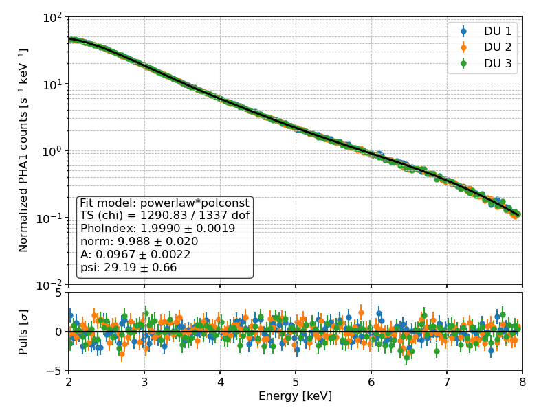
PHA1 (i.e., Stokes I) counts and best-fit spectral model for a toy example.
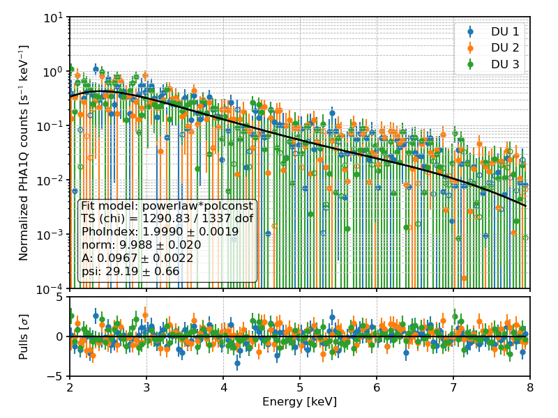
PHA1Q (i.e., Stokes Q) counts and best-fit spectral model for a toy example.
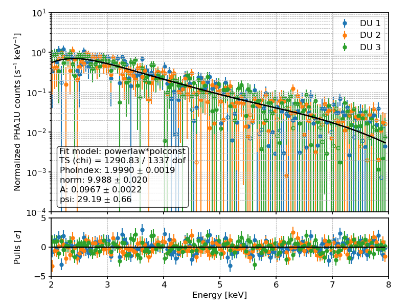
PHA1U (i.e., Stokes U) counts and best-fit spectral model for a toy example.
Alternatively, one can use the normalized Stokes parameters to factor out the spectral part and do a three-parameter purely-polarimetric fit. This will simultaneously fit the six normalized input files to the additive flavor of the constant polarization model returning the best-fit polarization degree and angle. (You should notice that the normalization, in this case, is a phony parameter to make the model additive and is set to 1 prior to the binning of the fit process.) It should be noticed that, in this case, the model is only folded with the modulation factor (as opposed to the modulation response function).
Warning
Beware that, statistically speaking, the treatment of the response matrix
in fitting the normalized Stokes parameters is non correct, and therefore
this should be considered discouraged and might be removed in a future
ixpeobssim version.